# The Math That Explains Why More Rabbits Means More Foxes — Then Fewer Rabbits
Here’s something that sounds like a riddle: why do rabbit populations boom, then fox populations boom, then rabbit populations crash, then fox populations crash — and then the whole cycle starts over again?
The answer is written in two equations from 1925. And the pattern they describe doesn’t just show up in forests. It shows up in economies, in neural circuits, in the dynamics of anything that hunts anything else.
This is the Lotka-Volterra model — and it’s one of the most surprisingly beautiful pieces of math you’ll ever see visualized.
—
The Counterintuitive Cycle
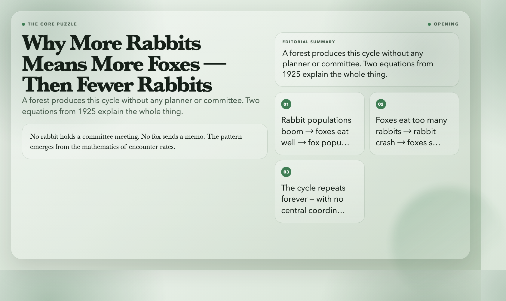
Imagine a forest with rabbits and foxes. When rabbits are plentiful, foxes eat well, raise more pups, and their population climbs. That’s obvious. But here’s the part that isn’t: when foxes are plentiful and rabbit populations start to fall, the fox population keeps growing anyway — because they’ve been eating so well. Only later do fox numbers crash, as starvation sets in.
Meanwhile, with fewer foxes around, rabbit populations recover. Then with more rabbits, fox populations start climbing again. Around and around it goes.
This creates a periodic oscillation — two populations chasing each other in a loop, like dancers following the same music.
The Hudson’s Bay Company kept records of rabbit and fox pelts traded across Canada from 1845 to 1935. When mathematicians plotted the data decades later, the cycle was unmistakable: it matched the Lotka-Volterra equations almost perfectly.
Try it yourself: the Lotka-Volterra Predator-Prey Model on ElysiaTools lets you set initial populations, growth rates, and watch the system evolve in real time. You’ll see the phase space diagram — a loop that traces exactly the path the ecosystem takes, over and over.
—
The Two Equations Behind the Rhythm
Here’s what the model says:
– Rabbits grow at a rate proportional to how many rabbits there are (more rabbits = faster breeding).
– Rabbits get eaten at a rate proportional to both rabbit and fox populations (more foxes + more rabbits = more meals).
– Foxes die at a rate proportional to how many foxes there are — starvation when prey runs out.
– Foxes reproduce at a rate proportional to how well they’ve been eating.
So:
“`
dRabbit/dt = a×Rabbit − b×Rabbit×Fox
dFox/dt = c×Rabbit×Fox − d×Fox
“`
The remarkable thing: just these two equations, with no hidden parameters and no central coordinator, produce the exact oscillation pattern found in real forests. No rabbit holds a committee meeting. No fox sends a memo. The pattern emerges from the mathematics of encounter rates.
—
Phase Space: Where the Beauty Lives
Most people picture this as a line graph — rabbit population over time, fox population over time, crossing and recrossing. But the phase space view is where the math gets visually stunning.
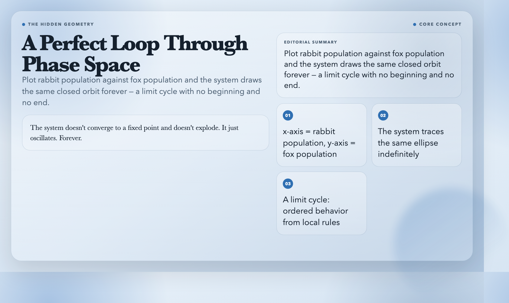
In the phase space, the x-axis is rabbit population and the y-axis is fox population. As the system runs, it traces a line through this space — and in the classic Lotka-Volterra model, that line closes on itself. It forms a perfect loop: the ecosystem travels around the same orbit, never settling down, never blowing up.
This is a limit cycle. The system doesn’t converge to a fixed point and doesn’t explode. It just oscillates. Forever.
The interactive visualization shows both views simultaneously. Adjust the initial populations or the growth rates, and you’ll see the orbit stretch, compress, or spiral inward or outward. The same equations produce every flavor of cyclical behavior.
—
Where Else This Shows Up
Ecologists were first to use this model. But the same mathematics of “X grows, Y follows, Y peaks, X crashes, X recovers…” describes systems that have nothing to do with animals:
– Business cycles: when the economy expands, companies invest and hire (prey boom); costs and defaults rise, recessions hit (predators eat prey); economy contracts; conditions recover. The Harrod-Domar model (1936) tried to put this math into macroeconomics.
– Neural circuits: excitatory and inhibitory neurons follow the same oscillatory structure. The 1972 Wilson-Cowan model formalized how two populations — one activating, one suppressing — produce the brain’s rhythmic oscillations from breathing to REM sleep.
– Epidemics: the SIR model (Susceptible → Infected → Recovered) is a direct cousin of Lotka-Volterra. When infected individuals are plentiful, recovery and death (predators) rise. When infected numbers fall, the predator declines. COVID-19’s waves followed dynamics that mathematicians recognized immediately as Lotka-Volterra with poor parameter estimates.
– Arms races: Frederick Lanchester published his combat model in 1916, showing two fighter squadrons hunting each other produce mathematically identical oscillations. Lewis Fry Richardson extended this to international conflict in 1935, coining “the war of the eatable and the eaters.”
In every case, the structure is identical: two populations where each one is changed by encounters with the other.
—
What the Model Doesn’t Tell You
Here’s what the classic Lotka-Volterra model doesn’t do: it never stops.
In the real world, rabbit and fox populations on an isolated island eventually settle down. The cycle dampens. The system reaches an equilibrium. The pure math never does. The loop goes on forever.
Real ecosystems add something the equations miss: density-dependent effects. When rabbits get too numerous, food runs out and disease spreads, limiting growth even without foxes. When foxes get too numerous, they eat so many rabbits that there’s not enough food for themselves. These feedback loops add damping terms — and that’s when the system spirals inward toward a stable point.
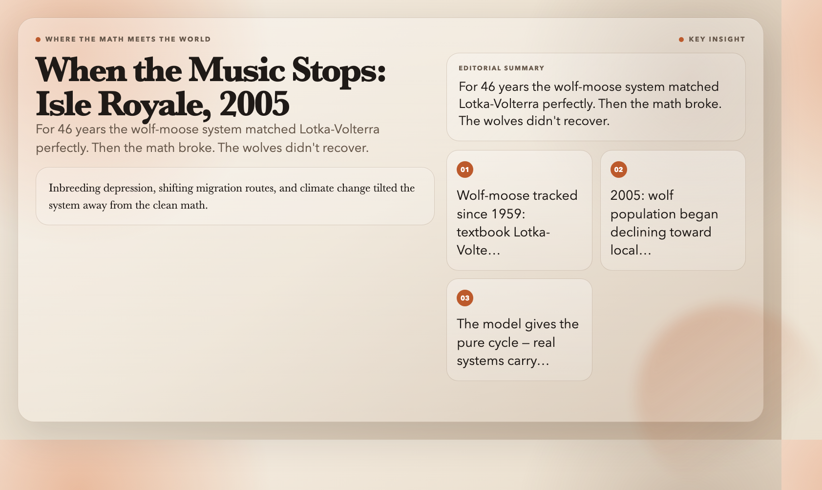
On Isle Royale in Lake Superior, biologists watched the wolf-moose cycle follow the textbook pattern for decades. Then, starting around 2005, the wolf population entered a long decline toward local extinction — inbreeding depression, shifting migration routes, and climate change tilted the system away from the clean math. The cycle dampened. The wolves may not recover.
This is the gap between the model and the world. The equations describe the pure logic of encounter — the skeleton of the cycle. But real systems carry extra baggage: disturbances, mutations, migrations, and shifts that can stop the music entirely.
The model cannot answer the question that matters: when does a system tip from oscillation into collapse? Math won’t tell you when the last wolf dies. It won’t tell you when the market stops cycling and starts cratering. It won’t tell you when the epidemic stops following the curve and breaks the curve.
That judgment falls to people — with incomplete data, in real time, with consequences they can’t fully calculate.
But you cannot hear when the music goes wrong until you know what the right music sounds like. Lotka-Volterra gives you the reference pitch. What you do with it is not a math question.
—
Explore the model yourself: the Lotka-Volterra Predator-Prey Model on ElysiaTools runs entirely in your browser, no sign-up, no installation. Adjust parameters, switch between time series and phase space views, and hear what a self-governing system sounds like when it runs exactly as designed.