The Hidden Pattern in Numbers That Catch Fraud — and It Looks Nothing Like You’d Expect

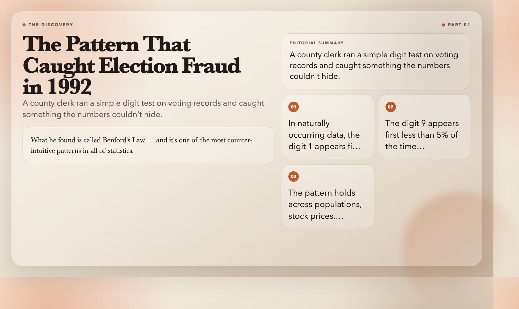
# The Hidden Pattern in Numbers That Catch Fraud — and It Looks Nothing Like You’d Expect

In 1992, a county clerk in Palmer, Pennsylvania ran a simple test on local election results. He wasn’t looking for anything sophisticated — just the distribution of first digits in the vote counts. What he found got the results thrown out and became one of the first documented cases of election fraud caught by pure mathematics.

The pattern he found is called Benford’s Law, and it’s one of the most counter-intuitive facts in all of statistics: in naturally occurring numerical data, the digit 1 shows up as the first digit about 30% of the time. The digit 9 shows up less than 5% of the time. This isn’t a glitch in the data — it’s a mathematical law, and once you see it, you can’t unsee it.

You can explore it interactively right now — no math degree required.

Why 1 Appears More Than 9

Imagine you’re standing at the start of a number line. As you count upward, you pass through 1, 2, 3… up to 9. Then what happens? You don’t go to 10. You go to 10 * 10 = 100. That’s a 10x jump.

Now think about this on a logarithmic scale — where each step is a multiplication, not an addition. On that scale, the distance from 1 to 2 covers 30% of the range from 1 to 10. The distance from 8 to 9 covers less than 5%.

So if you pick a random number from naturally occurring data, you’re more likely to land in that “1-zone” than the “9-zone.” The probability isn’t 11% for each digit (as random chance would suggest). Instead:

– 1 appears ~30.1% of the time
– 2 appears ~17.6%
– 3 appears ~12.5%
– …
– 9 appears only ~4.6%

This is Benford’s Law. And once you know it, you’ll start seeing it everywhere.

The Law of Cosines: The Formula Your Calculator Uses Without Telling You

Every triangle has secrets. The Law of Cosines is the tool that hides inside your calculator’s “solve triangle” button — and it’s more powerful than most people realize.

Given three sides of a triangle (a, b, c), the Law of Cosines finds any angle:

c² = a² + b² − 2ab·cos(C)

If C is a right angle (90°), cos(C) = 0, and the formula collapses into the Pythagorean theorem. This means the Law of Cosines is a generalization of every right-triangle calculation you’ve ever done.

The visualization lets you drag the vertices and watch the formula update in real-time. Try it: make one angle approach 90° and watch the formula converge. It suddenly clicks — the abstract becomes tactile.

Real-world uses include:

– Navigation systems calculating distances between GPS coordinates
– Architecture determining structural loads on angled supports
– Robotics planning the angle of a robotic arm’s reach

The step-by-step proof tab breaks the derivation into five stages. If you ever wondered why the Pythagorean theorem works — not just that it works — this is the interactive answer.

The Predator-Prey Model: How Populations Crash and Recover

Here’s a puzzle that stumped ecologists for decades: why do populations of lynx and hare fluctuate in clean, repeating cycles? The math that explains it was invented in 1925 by two scientists working completely independently.

Alfred Lotka (in the US) and Vito Volterra (in Italy) derived the same equations to describe a system where:

– More hares → more food → more lynx
– More lynx → more predation → fewer hares
– Fewer hares → less food → fewer lynx
– Fewer lynx → hares recover → cycle repeats

The equations look deceptively simple:

“dx/dt = ax − bxy (hare population) dy/dt = cxy − dy (lynx population)“

But what emerges is a closed orbit — populations trace out the same oval path over and over, like a marble rolling in a elliptical bowl. There’s no chaos here, no sensitivity to starting conditions. Give the simulator the same initial values and you get the same cycle every time.

You can explore three dynamics modes:
– Classic — closed orbits (periodicity)
– Damped — spirals inward (populations converge to equilibrium)
– Explosive — spirals outward (population explosion followed by collapse)

This model launched entire fields of mathematical ecology. It was one of the first times biologists used differential equations to predict natural systems — and it worked.

The Lorenz Attractor: The Butterfly That Causes Hurricanes

In 1961, Edward Lorenz was running a weather simulation. He wanted to repeat a run, so he typed in the starting values — but he only used three decimal places instead of six.

The result was completely different.

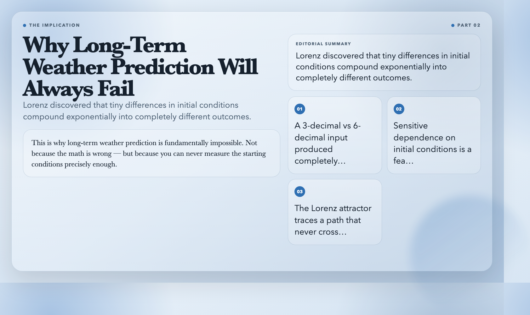
This wasn’t a computer error. Lorenz had discovered sensitive dependence on initial conditions — the hallmark of chaos. Tiny differences compound exponentially until the system becomes unpredictable.

The Lorenz attractor — that distinctive butterfly-shaped 3D trajectory — traces a path that never crosses itself and never repeats. It spirals around two “wing” regions, unpredictable yet bounded. You can set the three parameters (σ, ρ, β) and watch the trajectory shift from orderly loops to chaotic flutters.

The magic is in the numbers. Start with σ=10, ρ=28, β=2.67 (the classic values), and watch the butterfly form. Change ρ to 35 and the pattern shatters into apparent randomness. The attractor exists right at the edge of chaos — ordered enough to see structure, disordered enough to never repeat.

This is why long-term weather prediction is fundamentally impossible. Not because the math is wrong — but because you can never measure the starting conditions precisely enough.

The Logistic Map: Where Order Breaks Down Into Chaos

If there’s one visualization that changed how mathematicians think about prediction, it’s the logistic map. It’s a deceptively simple equation:

xₙ₊₁ = r · xₙ · (1 − xₙ)

Only one parameter: r. Only one variable: x. But as you increase r from 1 to 4, the behavior goes through every phase imaginable:

– r < 3: x settles to a single stable value
– r = 3.0 to 3.44: x oscillates between two values
– r = 3.45 to 3.54: x oscillates between four values
– r > 3.57: chaos — no pattern, no prediction possible
– r > 3.83: windows of order buried inside chaos

The bifurcation diagram makes this visible. Each vertical slice shows the long-term behavior of x for a given r. The forking structure reveals that chaos isn’t randomness — it has structure, just not the kind you can predict.

This is the Feigenbaum constant (δ ≈ 4.669…) — a number that describes how fast the period-doubling cascades occur, and it shows up in completely unrelated physical systems. Electrical circuits, fluid flows, chemical reactions — all follow the same sequence of bifurcations on the way to chaos.

The implication is uncomfortable: even systems that appear random might be perfectly deterministic. They just happen to be chaotic.

The Lotka-Volterra Difference: What Makes These Visualizations Different

You might be wondering: aren’t these just pretty math demos? Why would I use a web tool instead of just reading about these concepts in a textbook?

The answer is embodied understanding. The Law of Cosines generalizes the Pythagorean theorem — but when you drag a triangle’s vertex and watch c² equal a² + b², the relationship clicks. Predator-prey populations oscillate in theory. Watching the phase portrait spiral inward — seeing the system settle — makes it real.

These tools take concepts that exist in dense academic prose and let you feel them. The sliders for Lotka-Volterra parameters aren’t just UI chrome — they’re the actual variables that determine whether the system survives, explodes, or settles. Move the predation rate (b) from 0.1 to 0.4 and watch the orbit tighten. Something that felt abstract suddenly has texture.

The other thing these tools share: they’re built to fail gracefully. Try feeding Benford’s Law a list of uniform random numbers and the chi-squared test will reject it every time — exactly as expected. The tool isn’t trying to confirm your expectations. It’s a window into what the math actually says.

The Question Nobody’s Asking

We’ve built entire fields of knowledge around the assumption that enough data + enough computation = reliable prediction. The logistic map demolishes that assumption. It shows deterministic systems that look random — predictable in structure, unpredictable in outcome. The Lorenz attractor shows that sensitivity to initial conditions isn’t a flaw in our models; it’s a feature of nature. Benford’s Law goes further: it proves that natural data follows invisible rules, and those rules evaporate the moment someone fabricates numbers.

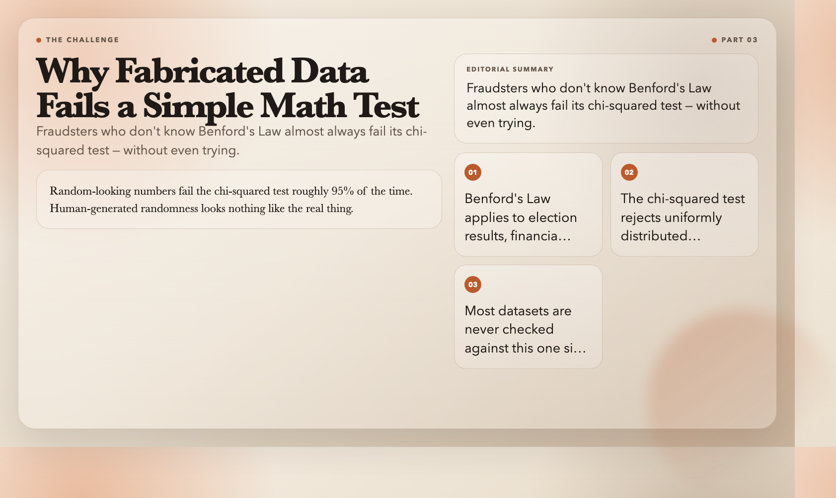
A fraudster who doesn’t know Benford’s Law will almost certainly fail it. Fabricated data fails the chi-squared test roughly 95% of the time — not because the test is sophisticated, but because human-generated “randomness” looks nothing like the real thing.

That’s the uncomfortable part.

Now think about every dataset you’ve trusted. Election results. COVID statistics. GDP figures. Academic research data. Climate records.

How many of them have been checked against Benford’s Law?

How many should have been?

The question isn’t whether Benford’s Law works. The question is why so few people in positions of power actually use it.

Every day, datasets get published, certified, and acted upon — election results, financial statements, scientific papers, pandemic figures. How many of them have been checked against this one simple pattern?