7 Interactive Chemistry Visualizations That Actually Make Concepts Click
You memorized VSEPR shape names for the exam. You balanced redox equations until they stuck. But ask yourself: when was the last time you watched a molecule actually rotate in 3D, or saw the exact pH where litmus changes from red to blue — not as a diagram, but as something you caused to happen?
Most chemistry education stops at the figure. These 7 interactive visualizations go further: you manipulate variables, watch reactions unfold in real time, and build the intuition that static textbook images never provided.
#
Acid-Base Indicators
Phenolphthalein flips from colorless to pink at pH 8.2. Methyl orange switches from red to yellow at pH 3.1. These aren’t arbitrary numbers — they define where an indicator is 50% protonated and 50% deprotonated, which is exactly when its color is in transition. Get that right, and your titration endpoint makes sense.
The Acid-Base Indicators visualization runs live titrations across four common indicators. Pick acid and base types, set initial concentrations, then watch the pH curve build drop by drop as titrant is added. The indicator color changes precisely within its transition range — no approximations, no hand-waving.

This is the difference between reading “phenolphthalein is colorless below pH 8.2 and pink above” and actually seeing it change color at pH 8.7, 9.0, 9.7 as you run a virtual strong acid-strong base titration. Students who struggle with buffer calculations often just need to see the plateau in the titration curve where pH resists change — and that’s exactly what this visualization makes visible.
#
VSEPR Molecular Geometry
VSEPR theory predicts molecular shapes from electron pair repulsion. The rule: electron pairs — bonding or non-bonding — orient to maximize the angles between them. Four electron pairs push into a tetrahedron (109.5°). Three bonding pairs with one lone pair compress to 107° in a trigonal pyramidal shape. Two bonding pairs with two lone pairs settle at 104.5° in a bent shape.
The VSEPR Model renders these geometries interactively in 3D. Choose a central atom, set bonding and lone electron pairs, then rotate the molecule with your mouse. Bond angles update numerically as you spin. Lone pairs display distinctly — they occupy space without anchoring an atom, which is precisely why they compress the angles other bonds form between them.
The visualization runs through common molecular shapes: linear (CO₂), trigonal planar (BF₃), tetrahedral (CH₄), trigonal pyramidal (NH₃), bent (H₂O), T-shaped (ClF₃), and more. When you can see water’s 104.5° bond angle versus ammonia’s 107°, and then explain why — lone pair repulsion — the theory stops being a memorization exercise and starts being something you understand.
#
Enzyme Kinetics
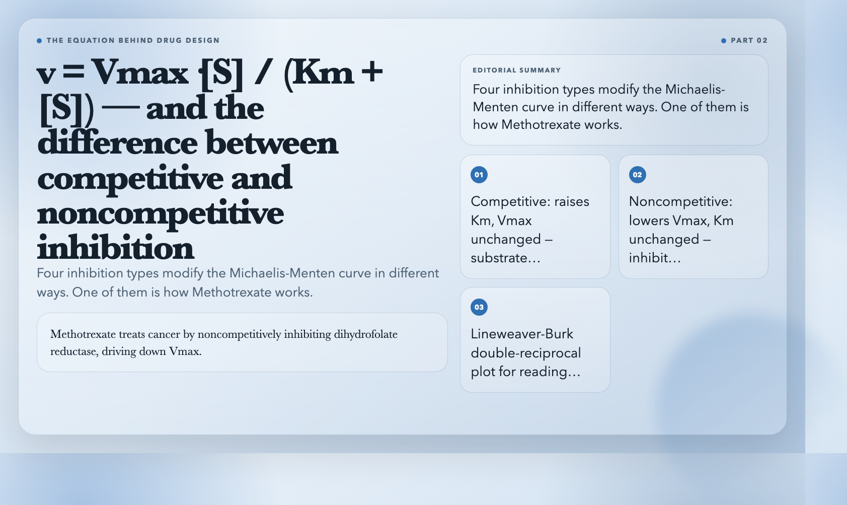
The Michaelis-Menten equation describes how enzymes work: v = Vmax·[S] / (Km + [S]). Vmax is the maximum reaction rate when the enzyme is saturated. Km is the substrate concentration at which reaction rate is half of Vmax. These two numbers characterize any enzyme-substrate pair.
The Enzyme Kinetics visualization plots this curve interactively as you adjust Vmax, Km, and inhibitor parameters. But it shows four inhibition types simultaneously — competitive, noncompetitive, uncompetitive, and mixed — each modifying the curve differently. Competitive inhibition raises the apparent Km but leaves Vmax unchanged. Noncompetitive lowers Vmax without touching Km. Uncompetitive does both.
In drug development, this matters directly. Methotrexate treats cancer by noncompetitively inhibiting dihydrofolate reductase, driving down Vmax for folate metabolism in fast-dividing cells. If you don’t know what noncompetitive inhibition looks like on a Michaelis-Menten plot, you don’t understand why the dosing schedule matters. The visualization makes that connection tangible.
#
Chromatography Principles
Chromatography separates chemicals by how quickly each component travels through a medium. Retention time is how long a component takes to emerge from the column. Resolution quantifies how cleanly two peaks separate. Theoretical plates measure column efficiency — more plates means sharper peaks and better separation.
The Chromatography Principles visualization builds a simulated chromatogram as you adjust parameters. Increase column length, and resolution improves but retention time lengthens. Decrease flow rate, and peaks sharpen but the run takes longer. Change the mobile phase composition, and peak positions shift in ways that aren’t always predictable without running the experiment.
Real-world chromatography optimization is a tradeoff tree: you improve resolution in one dimension and sacrifice it in another. The visualization lets you explore those tradeoffs freely. Run 20 virtual experiments in the time it would take to set up one real column.
#
Spectrophotometry
The Beer-Lambert Law governs light absorption: A = ε·c·l. Absorbance equals the molar absorptivity constant times concentration times path length. Measure absorbance at a known wavelength, and you can calculate concentration — the basis of quantitative chemical analysis.
The Spectrophotometry visualization demonstrates this with an interactive absorption spectrum. Set the wavelength, adjust solution concentration and cuvette path length, and watch the spectrum update in real time. Absorbance and transmittance display as inverse pairs — at 100% transmittance, absorbance is zero. At 50% transmittance, absorbance is 0.301.
A practical example: you dissolve a sample of unknown copper concentration in solution, measure its absorbance at 620nm (where Cu²⁺ absorbs maximally), and use a calibration curve of known standards to determine concentration. This is how environmental labs quantify heavy metal contamination in water. The visualization shows how each variable — wavelength selection, path length, concentration — feeds into that final measurement.
#
pH Calculator
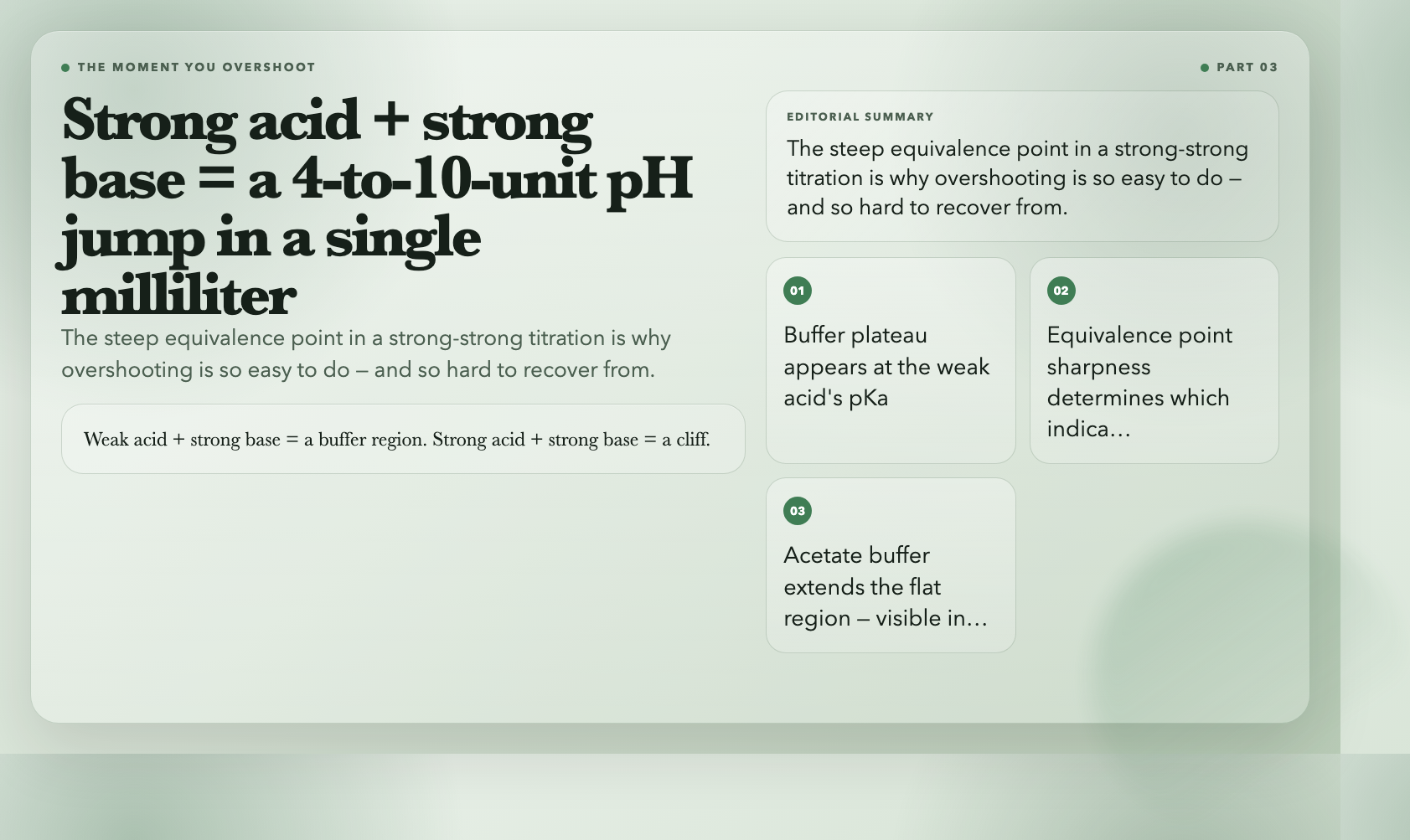
Strong acid and strong base titrations produce a steep pH jump near the equivalence point — often 4 to 10 units in a single milliliter. Weak acid and strong base titrations produce a gentler curve with a flatter buffer region around the weak acid’s pKa. These shape differences determine which indicator actually works.
The pH Calculator plots complete titration curves for any combination of strong/weak acids and bases. The curve for a 0.1M acetic acid (weak acid) titrated with 0.1M NaOH (strong base) shows a buffer region around pH 4.76 — the pKa of acetic acid. Add sodium acetate to create a true buffer, and the flat region extends noticeably. This is the plateau that resists pH change even when small amounts of strong acid or base are added.
If you’ve ever overshot a manual titration by accident and wondered why it happened so fast, the answer is in that steep equivalence point region. The visualization makes it impossible to miss.
#
Galvanic Cell
A galvanic cell converts chemical energy to electrical energy through spontaneous redox reactions. Zinc oxidizes at the anode, releasing electrons. Copper ions reduce at the cathode, consuming them. The standard cell potential for Zn|Cu is +1.10V — calculated from standard reduction potentials: E°(Cu²⁺/Cu) = +0.34V minus E°(Zn²⁺/Zn) = -0.76V.
The Galvanic Cell visualization simulates the full cell with adjustable electrode potentials, ion concentrations, and temperature. It calculates live EMF using the Nernst equation: E = E° – (RT/nF)·ln(Q). As the cell discharges and Cu²⁺ concentration drops at the cathode (plating out as solid Cu), the reaction quotient Q increases and the EMF decreases. This is why a real battery’s voltage drops as it discharges — the chemistry is visible in the numbers.
The visualization also shows electron flow in the external circuit and ion migration through the salt bridge, connecting the chemical and electrical perspectives on the same system.
#
Why These Work
Textbooks describe reactions. Visualizations let you break them.
Every concept here — pH indicator ranges, VSEPR bond angles, Michaelis-Menten kinetics, chromatographic resolution, Beer-Lambert absorbance, Nernst equation EMF — appears in standard chemistry curricula. The problem isn’t access to the information. The problem is that reading about something and feeling its behavior are different cognitive experiences.
Interactive tools collapse that gap. You can spend 20 minutes reading about how buffer capacity works, or you can load the pH calculator, add sodium acetate to acetic acid, and watch the plateau extend as you add small amounts of HCl. One approach gives you a definition. The other gives you a model you can reason with.
The 35 chemistry visualizations on ElysiaTools are free, browser-based, and require no account. Pick the concept that’s been giving you trouble. Run five experiments in five minutes. Come back to the textbook and see if it reads differently.