The Simple Math Behind Every Neural Network You’ve Ever Used

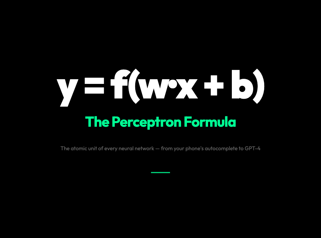
Every AI model you’ve ever interacted with — from the autocomplete in your phone to GPT-4 — runs on the same four-line formula. No jargon. No hand-waving. Just multiplication, addition, and a deliberate non-linearity that makes the whole thing work.

That formula is the perceptron, the fundamental computational unit of neural networks. And understanding it is the single biggest unlock in all of machine learning.

The Perceptron: y = f(w·x + b)

In 1958, Frank Rosenblatt built a machine he called the Mark I Perceptron. It was a physical device — wires, resistors, a camera — but the idea underneath was clean:

y = f(w¹x¹ + w²x² + w³x³ + … + b)

Where:

• x is what you feed in (an image’s pixels, a sentence’s tokens, a stock price)
• w is what the network has learned to “pay attention to” (weights)
• b is a learned threshold (bias)
• f is the activation function — and this is where everything interesting happens

The “w” learns *what to look at*. The “b” learns *when to care*. The activation function “f” learns *how to respond*.

This is a learnable feature transformer. That’s all a neuron is.

Why You Need an Activation Function

Here’s the part most tutorials skip.

Stack three perceptrons together without any activation functions. What do you get? Still a linear function. Still just w·x + b. You’ve spent three layers doing the same math as one.

Linear composition of linear = linear. No matter how deep your network, without non-linearity, you’re just drawing straight lines.

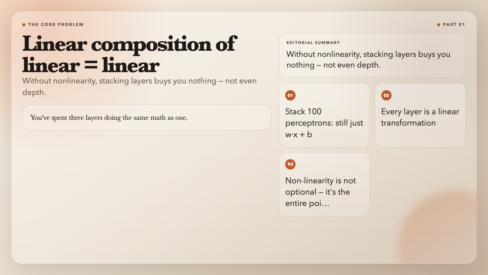
The activation function is what makes the network *curved*. And curved functions can learn curves — edges in images, semantic relationships in text, complex dynamics in physics.

That’s why activation functions exist:
1. Introduce nonlinearity so the network can learn complex patterns
2. Control the numerical range of outputs
3. Provide differentiability so backpropagation can work

Without them, you’re not training a neural network. You’re fitting a straight line.

The Activation Function Gallery

Different activation functions have different personalities. Here’s how to think about them:

Step Function (1958) — Rosenblatt’s original. Output 0 or 1. Great for theory, terrible for training. Gradients are either 0 or 1 with no in-between.

Sigmoid — Smoother. Maps any input to (0, 1). Easy to interpret as probability. But it has a gradient vanishing problem: for large inputs, the derivative approaches 0, so learning grinds to a halt in deep networks.

Tanh — Like sigmoid but maps to (-1, 1). Better for hidden layers because it’s zero-centered. Still suffers from vanishing gradients in deep networks.

ReLU (Rectified Linear Unit, 2011) — f(z) = max(0, z). Simple. Computationally cheap. Sparse activations. The gradient is 1 for positive inputs, 0 for negative ones. This was the breakthrough that made truly deep networks trainable.

Swish and GELU — Modern activation functions used in Transformers. Smooth, non-monotonic. GELU (used in BERT, GPT, T5) multiplies input by a sigmoid-weighted version of itself. Expensive, but makes large models significantly more stable.

The Gradient Vanishing Problem (And Why ReLU Fixed It)

Training a neural network means adjusting weights using backpropagation — propagating error gradients backwards through the network.

The gradient formula through a layer:

∂L/∂wᵢ = ∂L/∂y · f'(z) · xᵢ

If f'(z) ≈ 0, the gradient *vanishes*. No gradient, no learning. Simple as that.

For sigmoid: at large |z|, f'(z) → 0. Stack 10 layers with sigmoid activations and you get exponential decay of gradient signal. The early layers stop learning entirely. This was the deep learning deadlock.

ReLU broke the deadlock. For z > 0, f'(z) = 1. Gradient passes through unchanged. Deep networks could finally train.

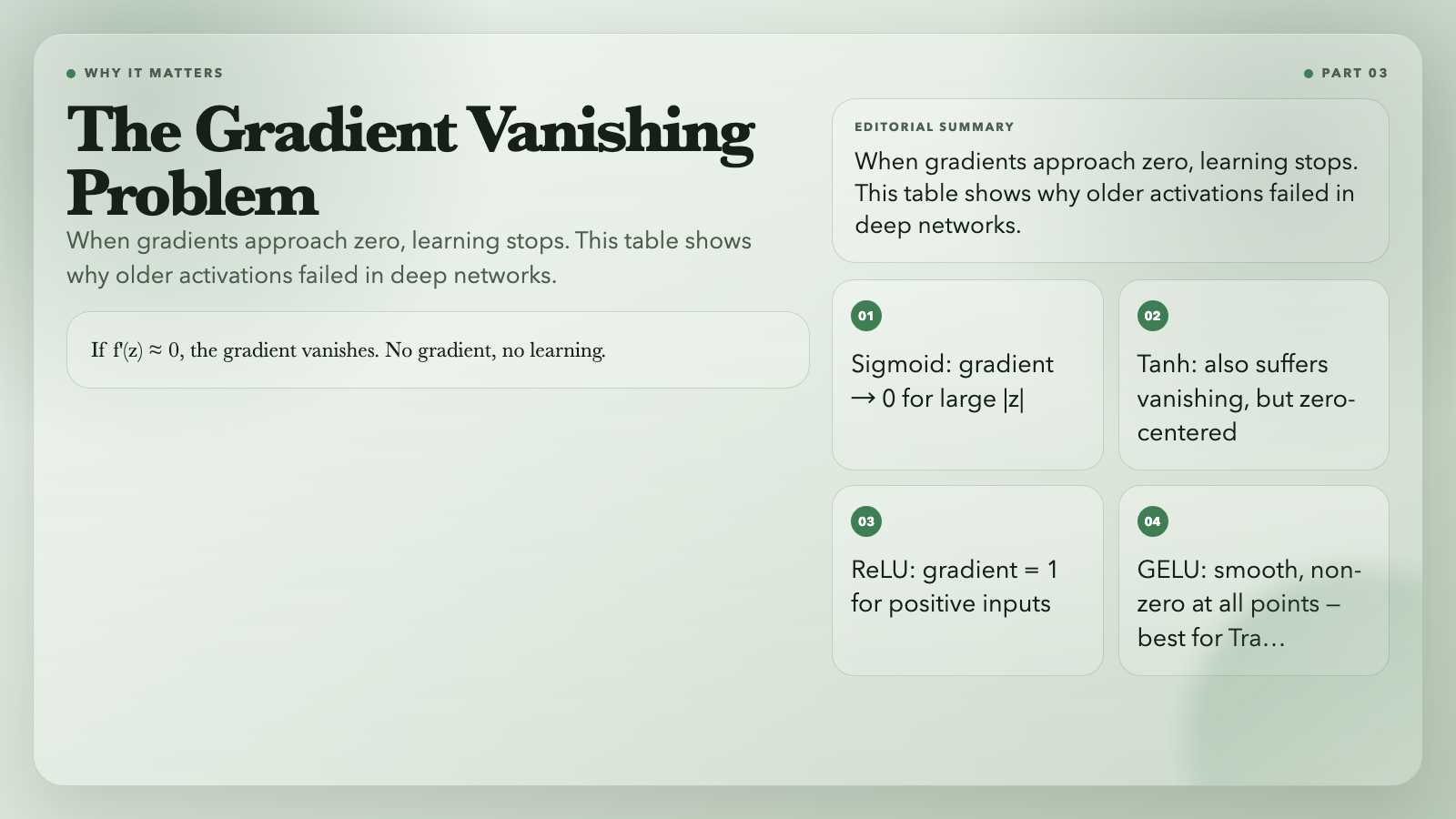
| Function | Large |z| Gradient | z=0 Gradient |
|—|—|—|
| Sigmoid | ≈ 0 (vanishing) | 0.25 |
| Tanh | ≈ 0 (vanishing) | 1.0 |
| ReLU | 1 (for z > 0) | 0 or 1 |
| GELU | Smooth non-zero | 0.5 |

The Universal Approximation Theorem (Why It Always Works)

Here’s the guarantee underneath everything: a feedforward network with *one* hidden layer can approximate any continuous function on compact subsets of Rⁿ, given enough neurons.

In practice, this means: if your network isn’t learning something, you probably need more neurons, better data, or better architecture — not a different fundamental approach. The perceptron framework is sufficient. That’s a remarkable fact.

What deep networks add is *efficiency*. Deeper networks can represent the same function with fewer parameters, using hierarchical feature composition.

Practical Rules for Choosing Activation Functions

For hidden layers in most architectures: ReLU is the default choice. It’s fast, simple, and rarely wrong.

For Transformers and modern large models: GELU. Used in BERT, GPT, T5, and most language models since 2017. The extra computation pays off at scale.

For binary classification output: Sigmoid — outputs a probability.

For multi-class classification: Softmax — ensures probabilities sum to 1.

For regression tasks: No activation (linear output).

Initialization matters too: ReLU pairs with He initialization. Sigmoid and Tanh pair with Xavier initialization. Mismatch initialization and activation, and your gradients start wrong.

What This Actually Means

Every time you use autocomplete, translate a sentence, or ask a model a question, you’re running thousands of perceptrons simultaneously — each one applying y = f(w·x + b), each one making a tiny nonlinear decision about what “features” to pass up the chain.

The magic isn’t mystical. It’s math. Specifically: it’s the deliberate injection of curvature into a stack of linear functions.

The perceptron is 67 years old. It’s still the atomic structure of every neural network in existence.

Try it yourself — adjust weights, switch activation functions, and watch the output change in real time:

Explore the Interactive Perceptron Visualization →

Or use the underlying tools directly to build, test, and understand these concepts programmatically:

• Perceptron Neuron Tool — Compute perceptron output with custom weights and activation functions
• AI Neural Network Diagram Generator — Visualize network architectures programmatically
• Backpropagation Deep Dive Visualization — See how gradients actually flow through a network

The math is simple. The implications are not. That’s the nature of interesting systems — simple rules, complex behavior. And the perceptron is the clearest example I know.