February 19, 2026
When a neural network predicts that an image shows a cat with 73% confidence, but it’s actually a dog, something has to tell that network: you were wrong, and here’s how wrong. That number — the thing that quantifies the gap between what the model predicted and what’s actually true — is called cross-entropy loss.
It’s the most commonly used loss function in machine learning. Every time you fine-tune a language model, train an image classifier, or build a recommender system, cross-entropy is almost certainly running behind the scenes, measuring the distance between the model’s beliefs and reality.
And yet, most developers who use it every day don’t really know what it means. Let’s fix that.
What Cross-Entropy Actually Measures
Cross-entropy measures the difference between two probability distributions: the true distribution (what actually happened) and the predicted distribution (what the model thinks happened).
Imagine you’re building a spam classifier. For a given email, the true distribution is simple — it’s either spam (100%) or not spam (0%). The model, however, might output something like 73% spam, 27% not spam.
Cross-entropy asks: if the model’s predictions were actually true, how much “surprise” would I experience on average? It quantifies this in bits or nats, depending on whether you use log base 2 or the natural log.
The formula looks intimidating in textbooks, but the intuition is straightforward: cross-entropy is high when the model is confidently wrong, and low when the model is confidently right.
Why Not Just Use Accuracy?
Accuracy is easy to understand — out of 100 predictions, how many were correct? But it’s a blunt instrument.
Consider two models making predictions on the same dataset:
- Model A: Confidently wrong on 5 samples (predicts 99% wrong class), correctly uncertain on 95
- Model B: Slightly wrong on all 100 samples (predicts 52% wrong class)
Both have 95% accuracy. But Model A has a much higher cross-entropy loss — it made confident mistakes that “cost” more. Model B, by contrast, knows it’s uncertain and is being appropriately cautious.
Accuracy doesn’t capture this distinction. Cross-entropy does. That’s why it’s the default loss for classification: it rewards honest uncertainty and punishes overconfidence.
The Math Nobody Reads
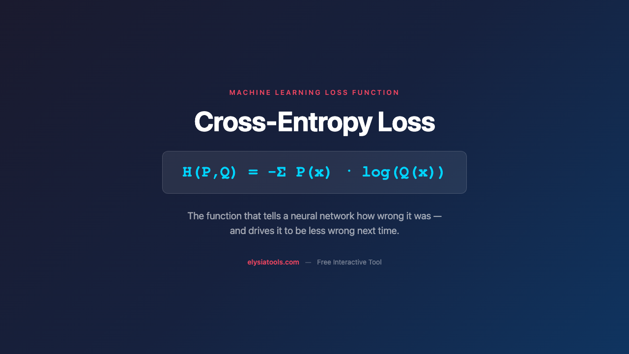
The cross-entropy H(P, Q) between a true distribution P and predicted distribution Q is:
H(P, Q) = -Σ P(x) · log(Q(x))For a binary classification problem where the true label is 1:
Loss = -log(predicted_probability_of_correct_class)When the model predicts 0.9 for the correct class, the loss is
-log(0.9) ≈ 0.105— a small error. When it predicts 0.1, the loss is
-log(0.1) ≈ 2.3— a large error. And when it predicts 0.001 (extremely confident and wrong), the loss spikes to
≈ 6.9.
This is the key property: cross-entropy loss grows dramatically when the model is confidently incorrect. It provides a strong gradient signal — the model learns much faster from being embarrassingly wrong than from being slightly wrong.
Why Softmax Makes Everything Positive
For multi-class problems, neural networks output raw scores (logits) for each class. The softmax function converts these into a probability distribution that sums to 1:
softmax(x_i) = exp(x_i) / Σ exp(x_j)The exponential function ensures all outputs are positive. The division ensures they sum to 1. This is crucial because cross-entropy needs valid probabilities — and because the exponential creates a “winner-take-all” effect that becomes more pronounced as the logits grow further apart.
Why this matters for training: when a model is very wrong, the softmax output becomes extreme (close to 1 for the wrong class). The resulting gradient is large, which means the model gets a strong signal to correct itself. As the model improves and predictions get closer to correct, the softmax outputs become less extreme and the gradients shrink — which is exactly what you want near a good solution.
Label Smoothing: Teaching Models to Be Humble
One problem with hard labels (0 for incorrect classes, 1 for the correct class) is that they can make models overconfident. A model trained on hard labels learns to output exactly 0 or 1, which means it never learns to say “I’m not sure.”
Label smoothing addresses this by replacing hard labels with soft ones. Instead of
[0, 0, 1]for a 3-class problem, you might use
[0.033, 0.033, 0.933]. The model still learns to prioritize the correct class, but it’s never pressured to be 100% certain.
This prevents overconfidence and often improves generalization — models that have seen smoothed labels tend to be better calibrated when they encounter data outside the training set.
Cross-Entropy vs. KL Divergence
Cross-entropy is closely related to KL divergence, and understanding the difference clarifies both:
H(P, Q) = H(P) + D_KL(P || Q)Where H(P) is the entropy of the true distribution, and D_KL(P || Q) is the KL divergence from Q to P.
Since the true distribution’s entropy H(P) is constant (it’s determined by the data, not the model), minimizing cross-entropy is equivalent to minimizing KL divergence. Both measures the “distance” between distributions, but KL divergence has a cleaner information-theoretic interpretation: it’s the extra surprise incurred by using Q to approximate P.
The practical difference is subtle but worth knowing: KL divergence is asymmetric (D_KL(P || Q) ≠ D_KL(Q || P)), which matters in some applications like generative models where you care about whether you’re being too conservative versus too permissive.
Numerical Stability: The Log(0) Problem
A naive implementation of cross-entropy can break when the model predicts exactly 0 for a class — because
log(0)is negative infinity.
The standard fix is the log-sum-exp trick. Instead of computing
log(softmax(x_i))directly (which requires computing exponentials that might overflow), you compute:
softmax(x)_i = exp(x_i – max(x)) / Σ exp(x_j – max(x))Subtracting the maximum logit from all values prevents overflow in the exponential. This trick appears in virtually every serious deep learning framework’s implementation of cross-entropy.
Why Temperature Matters
In softmax-based models, the temperature parameter T controls how “sharp” or “blurry” the output distribution becomes:
softmax(x/T)_i = exp(x_i/T) / Σ exp(x_j/T)With T = 1, you get the standard softmax. With T > 1, the distribution becomes more uniform (less confident). With T < 1, the distribution becomes sharper (more confident).
This is not just a training trick. Temperature scaling is used at inference time to calibrate model outputs — a model trained with temperature-aware loss can be adjusted post-hoc to produce more or less conservative predictions depending on the use case.
Try It Yourself
The Cross-Entropy Loss Visualizer on ElysiaTools lets you explore these concepts interactively. Adjust prediction confidence and see how loss changes. Experiment with label smoothing and temperature to understand their effects on the gradient signal. It’s a teaching tool, but also a sanity check — sometimes seeing the curve makes things click in a way that equations can’t.
The Bottom Line
Cross-entropy loss is not just “the thing we minimize during training.” It’s a carefully designed signal that shapes how neural networks learn. It rewards honest uncertainty, punishes confident mistakes, and provides strong gradients exactly when the model needs them most.
Every time you reach for a pre-trained model or train a classifier from scratch, cross-entropy is doing the invisible work of translating “wrong” into “how much wrong” — and that translation is why modern deep learning works as well as it does.