The One Number That Reveals Whether Any System Is Truly Predictable
Start with two identical coffee cups. Drop one. Fifteen minutes later, both are intact — the one you dropped and the one you didn’t. No difference. That’s a stable system.
Now try it with a double pendulum — two metal rods hinged together, swinging from the same point. Drop one. Fifteen minutes later, the one you dropped is spinning wildly in one direction; the other drifts lazily in another. Same initial conditions. Vastly different outcomes. That’s chaos — and it’s hiding in places you’d never expect.
The number that tells you which kind of system you’re looking at is called the Lyapunov exponent.
What the Exponent Actually Measures
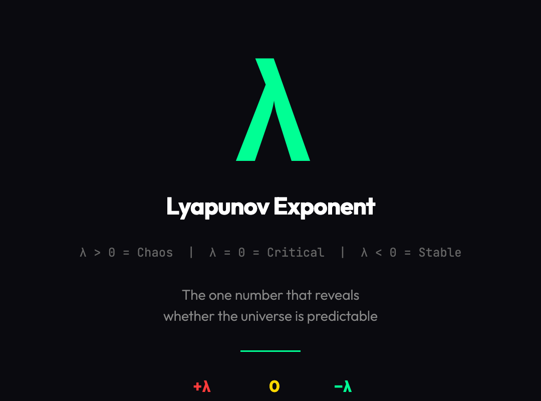
The Lyapunov exponent — denoted λ (lambda) — answers a deceptively simple question: if you start two nearly identical systems, how fast do they drift apart?
Mathematically, for a trajectory separation δx at time 0 evolving to δx(t) after time t:
λ = lim(t→∞) (1/t) · ln(|δx(t)/δx(0)|)
In plain English: take two starting points one ten-thousandth of a unit apart. Let the system evolve. Measure how much faster than exponential the separation grows. That’s λ.
λ < 0: Trajectories converge. The system is stable. Predictable. The double pendulum with heavy damping is λ < 0. So is a swinging door. So is your retirement portfolio in a bear market — it converges toward zero.
λ = 0: Trajectories maintain their separation. Periodic motion. A simple pendulum swinging at its natural frequency has λ = 0. The distance between two starting points stays constant forever.
λ > 0: Trajectories diverge exponentially. Chaos. The double pendulum without sufficient damping — the kind you see in physics demos — typically shows λ > 0. So does the Lorenz system. So does the weather.
The transition zone is what makes it interesting. For the logistic map — a deceptively simple recurrence relation used to model population growth — the Lyapunov exponent crosses from negative to positive at a parameter value of approximately 3.57. Below that, populations stabilize or oscillate predictably. Above it, they become chaotic. The entire behavior of a population model shifts based on a single parameter, and the Lyapunov exponent is what marks the boundary.
Why This Number Matters Beyond Physics
The Lyapunov exponent isn’t just a theoretical curiosity. It’s a diagnostic tool applied across disciplines.

Financial markets: Stock prices are often treated as random walks, but subtle Lyapunov analysis has shown that certain market regimes exhibit positive Lyapunov exponents — meaning extreme events are not random outliers but predictable consequences of sensitivity to initial conditions. The 1987 crash, the 1998 LTCM collapse, the 2008 crisis: all showed signatures that, in retrospect, were recoverable from Lyapunov-based early warning systems.
Biological systems: EEG readings from epilepsy patients show characteristic shifts in Lyapunov exponents before seizures — sometimes 15 to 30 minutes before the event. The brain transitions from a stable, λ < 0 regime to a临界 state where λ approaches zero, then briefly spikes positive during the seizure itself. This is being used experimentally to build seizure prediction devices.
Neural networks: The dynamics of recurrent neural networks (RNNs) can be characterized by their Lyapunov exponents. Networks with λ close to zero are at the “edge of chaos” — a regime where learning is most effective. This is why techniques like reservoir computing explicitly tune systems to this critical state.
Engineering: Power grids operate near critical transitions. A Lyapunov exponent analysis of grid frequency data can detect when the system is approaching instability — often minutes before a cascade failure becomes inevitable.
The Interactive Tool: Why You Should Try It
The Lyapunov Exponent visualization on ElysiaTools lets you explore this without reading a single equation.
You can select from four different systems: Logistic Map, Sine Map, Tent Map, and Hénon Map. Each exhibits different chaos properties. The Logistic Map is the classic period-doubling route to chaos — watch λ cross from negative to positive as you increase the parameter r from 2.5 toward 4.0. At r = 3.57, you’ll see the Lyapunov exponent hit zero for the first time — this is the onset of chaos. Push toward 4.0 and λ climbs above zero, staying positive.
What makes this visualization particularly valuable is that it doesn’t just show you the number — it shows you the trajectories themselves. Two nearly identical starting points diverge in real time. You can watch chaos happen.
The slider for initial separation (δx(0)) is especially instructive. Set it to 0.0001 and run the simulation. Then set it to 0.001 — ten times larger. The Lyapunov exponent should read the same. The trajectories should diverge at the same exponential rate. But notice what happens to the qualitative behavior: with a larger initial separation, the divergence becomes visible sooner, even though the underlying rate is identical.
This is the core insight: chaos is not about how far apart things end up. It’s about how fast the separation grows relative to the initial gap. A system with λ = 0.5 will, given enough time, separate two points that started 0.000001 apart just as dramatically as two that started 1 unit apart — the separation just takes longer in the first case.
The Butterfly Effect Isn’t What You Think

Edward Lorenz’s famous formulation — “does the flap of a butterfly’s wings in Brazil set off a tornado in Texas?” — is usually interpreted as: tiny causes have huge effects. But the Lyapunov exponent reveals a more precise picture.
A positive Lyapunov exponent doesn’t mean every perturbation grows without bound. It means the growth is exponential. For weather systems, λ ≈ 0.9 per day. That means a perturbation doubles in size roughly every 18 hours. After 10 days, that tiny butterfly wing flutter has amplified by a factor of roughly 65,000. After two weeks, it’s large enough to redirect a storm system.
The butterfly doesn’t cause the tornado. It shifts the initial conditions by a tiny amount, and the exponential divergence does the rest.
This is why long-range weather prediction is fundamentally impossible beyond approximately 10 to 14 days — not because our models are bad, but because any uncertainty in initial conditions (and there is always uncertainty) grows exponentially until it encompasses the entire phase space. At that point, all predictions are essentially random draws from the climate’s statistical distribution.
What λ = 0 Actually Means
The borderline case — λ = 0 — is often overlooked, but it’s arguably the most interesting regime.
At λ = 0, trajectories neither diverge nor converge. They maintain their separation. This is the signature of periodic motion — exactly periodic systems, where the same state repeats precisely. But it also describes systems at the edge of chaos: the critical points where phase transitions occur.
The 1/f noise spectrum found in many natural systems — from river flow to heartbeats to stock markets — often emerges at λ = 0. This is the regime of “pink noise,” neither fully predictable nor fully random. It’s the regime where complex, adaptive behavior emerges.
Tuning a system to λ = 0 — deliberately — is what makes reservoir computing work. A recurrent neural network at the edge of chaos can temporarily remember inputs, process them nonlinearly, and reproduce the computation with minimal interference from prior states. This is the sweet spot for computation.
The Deeper Implication
The Lyapunov exponent reveals something philosophically uncomfortable: many systems we assume are random are actually deterministic chaos. And many systems we assume are stable are actually metastable —λ is slightly positive, but the timescale of divergence is long enough that we mistake stability for predictability.
This has practical consequences. Insurance models that assume market returns are normally distributed miss the fat tails that emerge from slightly positive Lyapunov exponents. Medical models that assume heart rate variability is random noise are increasingly finding structured Lyapunov signatures that predict cardiac events. Economic models that treat consumer behavior as stochastic miss the sensitive dependence on initial conditions that creates wealth inequality.
The number λ doesn’t just tell you whether a system is chaotic. It tells you how predictable it is, how long your predictions remain valid, and how small an uncertainty in your initial knowledge becomes irrelevant over time.
And it turns out that many of the systems we care most about — economies, ecosystems, brains, power grids, climate — have λ just barely above zero. Not chaotic enough to look random on a chart, but not stable enough to predict with any precision over the long term.
That’s the real lesson of the Lyapunov exponent: the universe is not as predictable as Newton suggested, and not as random as quantum mechanics seems to imply. It’s something in between — sensitively dependent on initial conditions, but within bounds. Deterministic, yet only finitely predictable. Chaotic, but not without structure.
The number λ tells you exactly where on that spectrum any given system sits.
Try the interactive Lyapunov Exponent tool — pick a system, slide the parameter, and watch the trajectories diverge. It’s one of the more instructive five minutes you can spend if you want to understand why prediction is both possible and impossible, depending entirely on what you’re trying to predict.