If you’ve ever stared at a physics problem wondering which of the five SUVAT quantities you actually know, you know the bottleneck isn’t algebra — it’s figuring out which two unknowns the equations can solve for once you’ve pinned down the other three. The Physics Kinematics Problem Solver takes that decision off your plate: enter any three of displacement, initial velocity, final velocity, acceleration, or time, and it walks you through finding the other two with the formula, the substitution, and the result all spelled out. The same interface flips into projectile mode for launch speed, angle, and height, returning range, time of flight, and apex height with the same step-by-step derivation. That last 10% — the part where you check whether your answer even makes physical sense — is where a solver earns its keep.
But a tool like this is only useful if you understand what it’s solving. Kinematics has a reputation for being mechanical, and at the surface it is: four short equations, one algebraic identity, a handful of sign conventions. The reason it still trips people up isn’t the math — it’s the modeling choices: when is the acceleration constant? Which direction counts as positive? How do you handle a projectile whose launch and landing heights don’t match? This guide walks through the kinematics toolkit end to end, then shows how to feed it into the solver cleanly so you spend your time on the physics, not the arithmetic.

What “kinematics” actually means
Kinematics is the part of mechanics that describes how objects move, leaving why to dynamics. You treat position, velocity, and acceleration as functions of time and connect them through a small set of relations. No forces enter the picture. That separation is what makes kinematics tractable: the equations are just definitions stacked on top of each other, and as long as the acceleration stays constant over the interval you’re studying, the answers are exact, not approximate.
The standard toolkit rests on four equations, usually called the SUVAT equations because each variable has a single capital letter:
- s — displacement (change in position, signed)
- u — initial velocity (velocity at the start of the interval)
- v — final velocity (velocity at the end of the interval)
- a — acceleration (assumed constant over the interval)
- t — time elapsed over the interval
The four relations among them, under constant acceleration, are:
- v = u + at
- s = ut + ½at²
- s = ½(u + v)t
- v² = u² + 2as
Notice that no single equation contains all five variables. That isn’t a coincidence — it’s why the textbook version of the problem always tells you “three quantities are known, find the other two.” Pick two equations that share the unknown you want, eliminate the other unknown, and you have your answer. In practice this is fast if you know the equations cold and infuriating if you don’t.
The Physics Kinematics Problem Solver automates the algebra step so the only thinking left is the modeling: which numbers go into the solver, which sign convention you’re using, and which answer is physically reasonable.
The five variables and why three is the magic number
With five unknowns (s, u, v, a, t) and four equations, the system is underdetermined by one variable. Specifying any three quantities uniquely fixes the other two — that’s the standard “given three, solve for two” rule. The complication is that not all triples are equally friendly: if you give the solver (s, u, t) it can find v and a cleanly, but if you give it (s, v, t) it needs a quadratic in u. Same answer, different algebra.
The trick is choosing which pair of unknowns is the easiest target. Most physics problems are written in one of these shapes:
- Free-fall style: you’re given the drop height (s), the initial velocity (usually zero, so u = 0), and one of v or t. You solve for the other.
- Braking problem: you’re given the initial speed (u), the stopping distance (s), and asked to find the deceleration (a) or the time to stop (t). Often v = 0 is implicit.
- Acceleration phase: you’re given u, a, and t, asked to find v and s — the simplest case, two direct substitutions.
Each of these collapses to a single pair of SUVAT equations. The solver walks through the selection so you can see which equations it picked and why, which makes it a useful study aid even when you don’t strictly need the arithmetic done for you. If you want to validate that your own approach matches the solver’s, run both and compare the substitution steps.
Sign conventions: the part students actually lose points on
The SUVAT equations don’t care about direction, but you do. The standard convention is to pick one direction as positive — usually “right is positive” or “up is positive” depending on the problem — and then write every signed quantity with that convention in mind. Gravity is then negative if you’re using up as positive, which is why a dropped ball has u = 0, a = -9.81 m/s², and a negative final velocity just before it hits the ground.
Two common pitfalls:
- Mixing conventions mid-problem. You start with up positive for the rise, then forget to flip the sign for the descent. The magnitude of the velocity is the same; the sign tells you direction.
- Forgetting that s is displacement, not distance. A ball thrown straight up and caught at the same height has s = 0 over the round trip, even though it traveled a positive total distance. This matters when you apply v² = u² + 2as: at the apex, v = 0 and s equals the maximum height, which you can solve for. But if you use total distance instead of displacement, the same equation gives a wrong answer.
The Physics Kinematics Problem Solver lets you sign your inputs explicitly, so if your acceleration is downward and you’ve taken up as positive, you write a = -9.81 rather than 9.81. The substitution step then shows the sign carried through correctly, which is exactly the kind of feedback that prevents the most common mistakes on exams.

Projectile motion as two independent kinematics problems
The moment an object leaves a surface — kicked, launched, thrown — it becomes a projectile. The defining feature of projectile motion is that the horizontal and vertical components of motion are independent of each other. The horizontal component experiences no acceleration (ignoring air resistance), so it moves at constant velocity. The vertical component is in free fall, with acceleration g pointing downward.
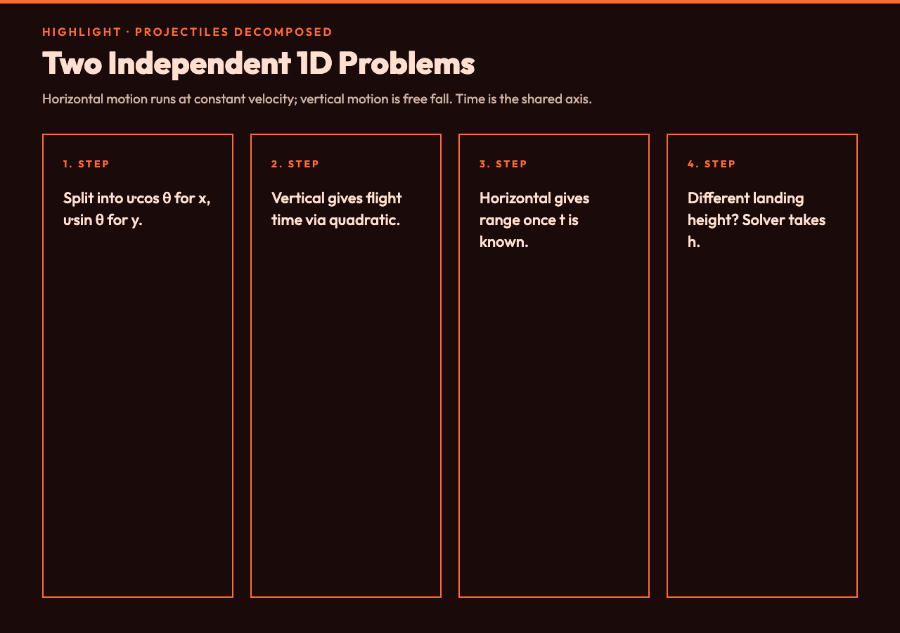
This independence is the single most important idea in projectile motion. It lets you split a 2D problem into two 1D problems:
- Horizontal: u_x = u cos θ, v_x = u_x (constant), s_x = u_x · t. Solve for range, time, or any horizontal quantity.
- Vertical: u_y = u sin θ, a_y = -g, then apply SUVAT vertically. Solve for max height, time of flight, or impact velocity.
The shared variable is t — the time of flight. Once you find t from the vertical equation, you feed it into the horizontal equation to get the range. The solver handles this by switching to a “projectile” mode where you enter launch speed, launch angle, and (optionally) initial height; it returns time of flight, range, and maximum height in one shot, with the two component problems shown separately in the derivation.
When the projectile lands at a different height than it launched
The textbook version assumes the projectile lands at the same height it launched from, which makes the time of flight 2u sin θ / g. Real problems don’t always oblige: a ball thrown off a cliff, a package dropped from a plane, a rocket launched from a hill. In these cases the landing height is different and you have to solve a quadratic for the time of impact.
The vertical displacement is s_y = u sin θ · t − ½ g t². If the projectile lands a distance h below the launch point, s_y = −h (negative because the landing height is below the launch). Plugging in:
−h = u sin θ · t − ½ g t²
½ g t² − u sin θ · t − h = 0
That’s a quadratic in t. Use the quadratic formula:
t = [u sin θ + √((u sin θ)² + 2 g h)] / g
(Take the positive root; the negative root is unphysical.) Once you have t, the horizontal range is x = u cos θ · t. The solver accepts an initial height parameter so you can skip the quadratic entirely — but knowing the derivation means you can sanity-check the answer when the textbook gives you a result that looks suspicious.
Putting it together: a worked example
A soccer ball is kicked from ground level with initial speed 18 m/s at an angle of 32° above the horizontal. How far does it travel before landing, and what is its maximum height?
Step 1: split the initial velocity.
u_x = 18 cos 32° ≈ 15.26 m/s
u_y = 18 sin 32° ≈ 9.54 m/s
Step 2: time of flight. Since the ball lands at the same height it launched from, t = 2 u_y / g = 2 × 9.54 / 9.81 ≈ 1.94 s.
Step 3: range. x = u_x · t = 15.26 × 1.94 ≈ 29.6 m.
Step 4: max height. At the apex, v_y = 0. Use v² = u² + 2as with v = 0: s = u_y² / (2 g) = 9.54² / (2 × 9.81) ≈ 4.64 m.
You can replicate this in the Physics Kinematics Problem Solver by switching to projectile mode, entering 18 for the speed, 32 for the angle, and 0 for the launch height. The solver returns range, time of flight, and max height, with the vertical and horizontal component derivations laid out side by side.
Common mistakes and how the solver catches them
Three mistakes show up over and over in kinematics problems:
- Using g = 9.81 when the problem is in feet. If the problem uses imperial units, g ≈ 32.2 ft/s². The solver accepts unit-agnostic input, but you still need to be consistent: either convert all quantities to SI first, or use imperial throughout.
- Treating a changing acceleration as constant. A car that accelerates, holds speed, then brakes is not a single-interval kinematics problem — it’s three, each with its own a. The solver is built for one interval at a time; for multi-stage problems, run it once per stage.
- Forgetting that v² = u² + 2as is sign-blind on the v term. If v and u have opposite signs, this equation breaks down because squaring erases the directional information. Use v = u + at or s = ut + ½at² instead when the signs differ.
The solver’s substitution step surfaces each of these. If you typed g = 9.81 in a problem stated in feet, the resulting range will look absurdly large — the solver won’t catch the unit mismatch, but the magnitude will be off by a factor of 3.28, which is hard to miss.
Why a step-by-step derivation beats a black-box answer
Most kinematics calculators give you the final answer with no work shown. That’s fine for a sanity check on a homework problem, but it doesn’t help you learn the method. The Physics Kinematics Problem Solver takes a different approach: every step of the substitution is shown explicitly, from the formula chosen to the values plugged in to the arithmetic simplification. You can read the derivation top to bottom and reconstruct the algebra yourself.
For a student, this means the tool doubles as a study aid. If you understand the underlying equations but keep making algebra errors, the solver confirms the right answer and shows you where your work diverged. If you don’t yet understand which equations apply, the solver’s choice of which two SUVAT equations to combine tells you the strategy you should have taken — and on the next problem you can try predicting that choice before reading what the solver did.
For an instructor, the same derivation is a useful template for worked examples in class or in problem sets. The structure — pick two equations, eliminate the unknown, substitute, simplify — is exactly the structure you want students to internalize, and having it spelled out line by line makes the reasoning visible.
How the solver handles edge cases
A few edge cases come up often enough to be worth thinking about:
- Negative time. If your inputs imply t < 0, the solver flags it. Physically, time can’t run backward, so this almost always means a sign error or a misinterpretation of which event is “initial” and which is “final.”
- Zero acceleration. If a = 0, two of the SUVAT equations degenerate (the v² = u² + 2as equation still works, but v = u + at is trivially true). The solver handles a = 0 gracefully and falls back to the equations that remain meaningful.
- Landing below the launch point in projectile mode. The solver accepts a negative initial height to model launches from elevated positions, and uses the quadratic form of the time-of-flight equation rather than the simplified 2u sin θ / g form.
- Degenerate projectile (vertical launch). If θ = 90°, the horizontal component is zero and the projectile goes straight up. The solver reports range = 0 and computes the apex and landing time using only the vertical equations.
These edge cases are precisely where most homework mistakes originate, so having a tool that handles them consistently is more valuable than it might first appear.
When kinematics stops being enough
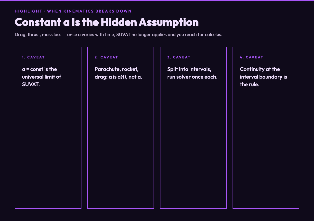
Kinematics assumes constant acceleration. Once a becomes a function of time — say, a rocket burning fuel and losing mass, or a falling object with significant air resistance — the SUVAT equations no longer apply. You need calculus: integrate a(t) to get v(t), integrate again to get s(t).
The boundary between “solvable with kinematics” and “needs calculus” isn’t always obvious. A skydiver before opening the parachute is approximately in free fall (a ≈ g), so kinematics applies. After the parachute opens, drag dominates and the acceleration is no longer constant — kinematics gives way to differential equations. The solver’s constant-acceleration assumption is the right tool for the first regime and the wrong tool for the second, which is itself a useful learning moment: knowing the limits of a method is part of understanding the method.
If you find yourself trying to feed the solver quantities that imply changing acceleration — for example, separate accelerations at different phases — split the motion into intervals and run the solver once per interval. Each interval has its own constant a, its own u and v (continuity at the boundary if the velocity is continuous, a jump if there’s an impulsive event like a collision), and its own s and t.
Putting the solver in a workflow
A reasonable workflow for a physics homework problem looks like this:
- Read the problem, identify the interval you’re studying, and write down which of s, u, v, a, t you know.
- Pick your sign convention (usually up or right is positive).
- Convert all quantities to consistent units (SI is the safest default).
- Hand-derive the answer using the SUVAT equations you think apply.
- Run the Physics Kinematics Problem Solver with the same inputs and compare.
- If the answers agree, you’ve checked your algebra. If they disagree, work through both derivations until you find the divergence.
The point isn’t to outsource the work — it’s to add a reliable second opinion. Used this way, the solver is a study aid that catches errors early and reinforces the right approach, rather than a black box that produces an answer without context.
Closing thoughts on a deceptively simple toolkit
Kinematics is one of those topics that looks shallow until you try to teach it. The equations are short, the algebra is tractable, and the problems feel repetitive after the first few. What the subject is actually training is the modeling instinct: deciding what counts as a system, what’s constant and what’s changing, where the boundaries are between intervals, and which signs go where. The arithmetic is the easy part. The thinking is the hard part.
A solver like this one is most valuable when it lets you skip the easy part and focus on the hard part. Run it as a check, not a replacement. Compare its derivation to yours. Read the substitution steps to see if you would have made the same choices. When the answers disagree, the disagreement is usually a sign error or a modeling decision — and either way, you’ve found something worth thinking about.
Open the Physics Kinematics Problem Solver, try the example above, and then try a problem from your own course material. The first time the solver confirms an answer you’ve wrestled with, you’ll understand exactly why a step-by-step derivation is more useful than a black-box number — and the next time you tackle a kinematics problem, you’ll find yourself reaching for the SUVAT equations with more confidence. The kinematics solver runs entirely in the browser, so it’s there whenever you need a second opinion — at the desk, in the library, or right before an exam.
Explore more free browser-based problem solvers at elysiatools.com.