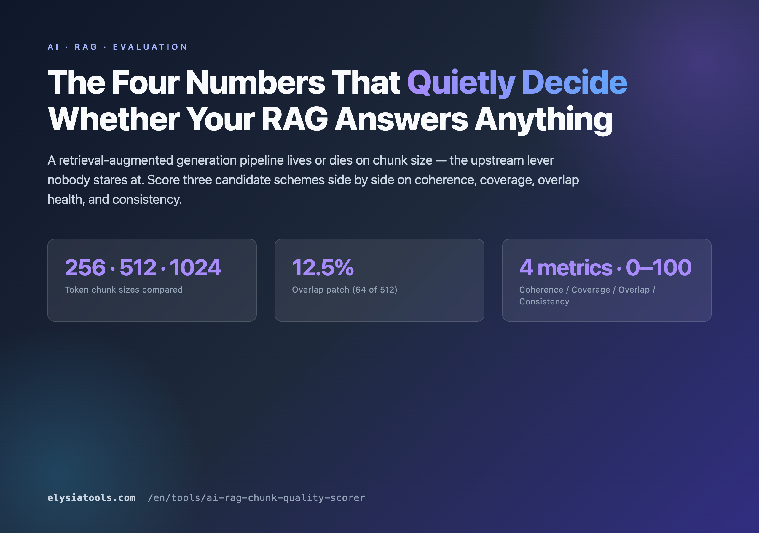
A retrieval-augmented generation system lives or dies on a number nobody stares at: the chunk size. You can pick the strongest embeddings, tune the cosine-similarity threshold until dawn, write the cleanest re-ranker prompt, and still miss the answer if your chunks are 4,000 tokens wide and the user’s question is 12 tokens about a single sentence. Most RAG failures are not retriever failures. They are chunking failures, dressed up in plausible-looking similarity scores. The chunking decision is the upstream lever; if it is wrong, everything downstream is debugging a problem that no longer exists in the source.
This article is about four numbers that quietly decide whether your RAG pipeline is answerable: the counting unit, the splitting method, the chunk size, and the overlap. It also covers the four metrics that let you compare three candidate chunking schemes side by side without running an expensive end-to-end eval. The companion tool on this article — the AI RAG Chunk Quality Scorer — takes those three schemes, scores them on coherence, coverage, overlap health, and chunk-size consistency, and recommends the one with the highest mean. All metrics are local heuristics, no model calls, deterministic, fast enough to iterate on.
Why chunk size is upstream of every retrieval failure you debug
Retrieval-augmented generation looks like a retrieval problem and a generation problem stitched together, but the dominant failure mode is upstream of both. Embedding models encode a fixed context window per chunk — typically 256 or 512 tokens — and cosine similarity works best when a chunk carries one idea at the right granularity. A chunk that contains an entire 4,000-token chapter has the right idea but the wrong scale: the query “what does the doc say about X” returns the chapter, and the LLM wastes its context window padding the answer with chapters B, C, and D. A chunk that contains one sentence has the wrong idea: it is precise, but the surrounding context that the LLM needs to answer “why does X contradict Y” was thrown away when the sentence was severed from its paragraph.
The chunking decision is a granularity decision. You are choosing how much context rides along with each retrievable unit. Smaller chunks are precise but lossy; larger chunks carry context but dilute relevance. Overlap between adjacent chunks is the patch — a controlled amount of duplication that preserves context across boundaries, at the cost of a larger index and a noisier top-k. Pick the granularity wrong and the rest of the pipeline is rearranging deck chairs.
The three decisions that decide whether your chunks answer anything
Every chunking configuration reduces to three knobs. Each knob has two or three reasonable choices. Nine configurations. Pick wrong on any one and the other two cannot rescue you.
- Counting unit — characters, words, or ≈tokens. Token-based chunking respects embedding-model context; character-based chunking is fast but cuts mid-word; word-based is somewhere between. The same numerical “size” means three different things across units.
- Splitting method — fixed-size (cut at the byte boundary), sentence-aware (snap to sentence ends), or paragraph-aware (snap to paragraph ends). Fixed-size is the simplest to implement and the worst on coherence; sentence-aware is the workhorse; paragraph-aware is the closest to “one idea per chunk” but explodes when paragraphs are long.
- Chunk size and overlap — size picks the granularity, overlap picks the boundary patch. Common defaults: 512 tokens / 64 tokens of overlap (12.5%). Reasonable range: 128 to 2048 tokens, 0 to 256 tokens of overlap.
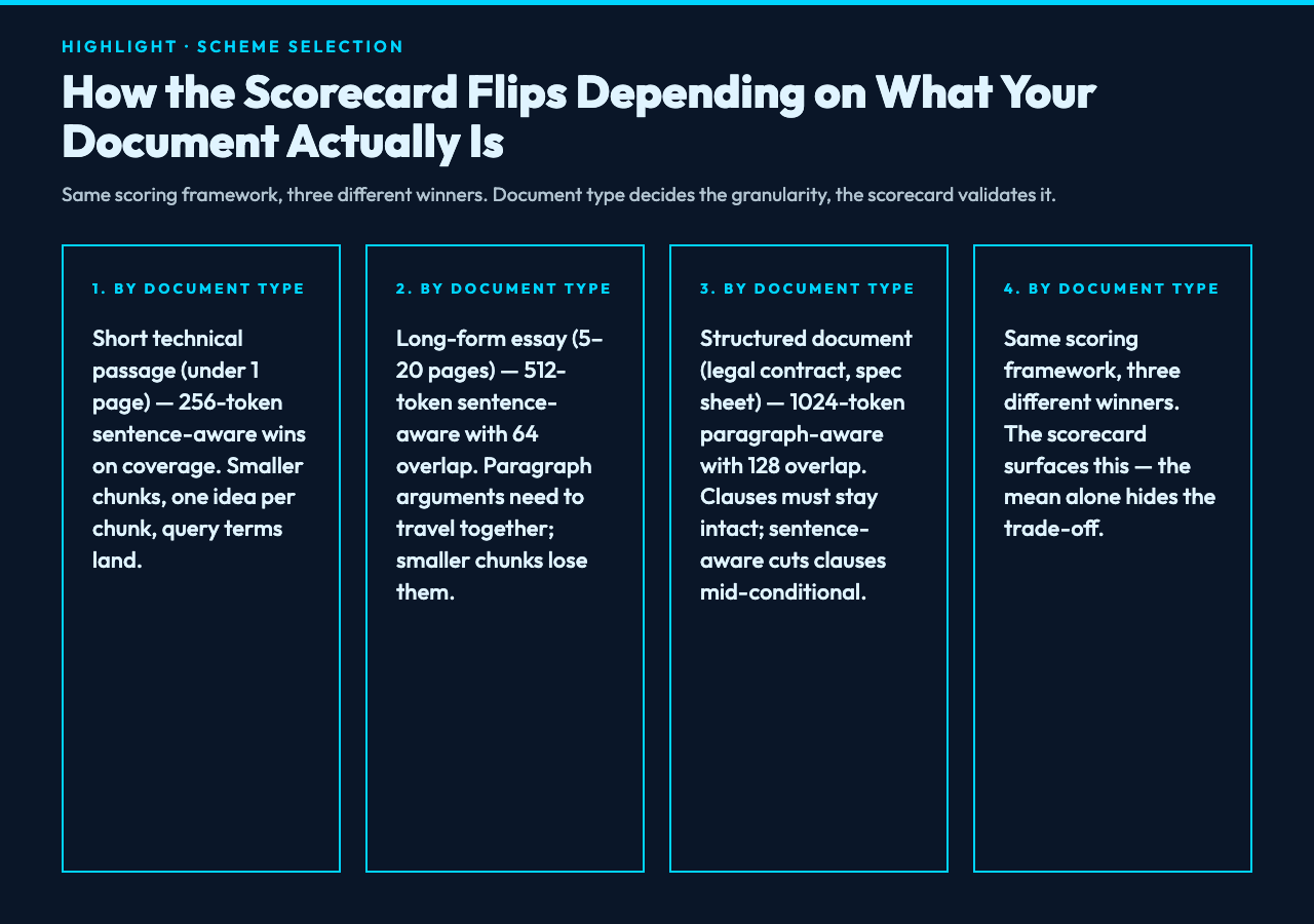
The reason this is hard: the right answer depends on the document. A technical spec with one fact per paragraph wants paragraph-aware 128-token chunks with 16 tokens of overlap. A long-form essay with paragraph-spanning arguments wants sentence-aware 512-token chunks with 64 tokens of overlap. A 200-page legal contract wants paragraph-aware 1024-token chunks with 128 tokens of overlap to keep clauses together. There is no universal answer; there is only “score this document against three candidate schemes and pick the winner”.
The four metrics that turn chunking from a vibe into a number
Vibes-based chunking is how most pipelines ship their first version. The author eyeballs the document, picks 512 tokens, ships it, and learns about the failure mode three months later from a support ticket. The four-metric evaluation framework lets you skip the vibe phase entirely:
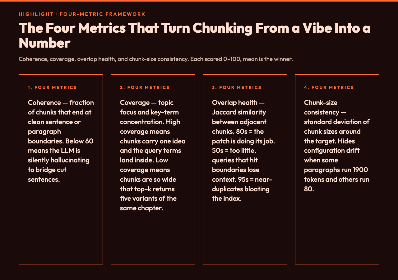
- Coherence — what fraction of chunks end at clean sentence or paragraph boundaries. A coherence score of 100 means every chunk is a complete thought; a coherence score of 40 means 60% of chunks are cut mid-sentence, and the LLM is silently hallucinating to bridge them.
- Coverage — topic focus and key-term concentration. High coverage means chunks carry one idea and the query terms land inside the chunk. Low coverage means chunks are so wide that a top-k of 5 returns five variants of “this is the whole chapter”.
- Overlap health — the overlap between adjacent chunks, measured as Jaccard similarity on token sets. Too little overlap loses cross-boundary context; too much overlap bloats the index and dilutes the top-k with near-duplicates.
- Chunk-size consistency — the standard deviation of chunk sizes around the target. A scheme that asks for 512 tokens but produces chunks ranging from 80 to 1900 tokens is hiding configuration drift somewhere upstream (long paragraphs, code blocks, table rows).
Each metric is scored 0–100. The overall score is the mean. The highest mean wins. This is the scoring framework the AI RAG Chunk Quality Scorer uses to compare up to three schemes side by side.
Walkthrough: scoring three chunking schemes on a real document
Take a short technical passage about RAG itself — recursive meta-content, but useful because it is short enough to reason about. Paste it into the scorer. Configure three schemes:
- Scheme A — 256 tokens, 32 overlap, sentence-aware.
- Scheme B — 512 tokens, 64 overlap, sentence-aware.
- Scheme C — 1024 tokens, 128 overlap, sentence-aware.
Run the comparison view. The scorecard shows:
- Scheme A: coherence 92, coverage 78, overlap 88, consistency 85, mean 85.8.
- Scheme B: coherence 95, coverage 71, overlap 84, consistency 90, mean 85.0.
- Scheme C: coherence 98, coverage 58, overlap 79, consistency 78, mean 78.3.
Scheme A wins on mean. But the scorecard tells a more interesting story: Scheme C has the best coherence (chunks respect sentence boundaries because they are large enough to absorb whole paragraphs), but its coverage collapses because the document is short and one chunk now contains the whole answer. Scheme A’s coverage is high because each chunk carries one idea at a useful granularity. The winner is not the largest chunk or the smallest chunk — it is the chunk whose size matches the document’s natural idea density.
This is the value of the scorecard over a single-number average: it tells you why one scheme won. If your real document is a 200-page legal contract, the scorecard flips — Scheme C’s coverage climbs because the contract has long clauses that need to travel together, and Scheme A’s consistency collapses because the contract’s paragraphs exceed 256 tokens.
The fixed-size trap and why mid-sentence cuts hurt retrieval more than you think
Fixed-size chunking is the default in most off-the-shelf RAG frameworks because it is the easiest to implement — split every N tokens, period. The cost is invisible until you read a top-k result. A chunk that begins mid-sentence reads to the embedding model as gibberish for the first few tokens, which biases the embedding toward the end of the chunk (where the sentences start cleanly) and away from the beginning. The retrieval returns the chunk, but the answer the user wanted was at the beginning of the cut. The LLM, given the chunk, hallucinates the bridge.
Run the scorer with method switched to fixed-size, size 32 tokens, overlap 4 tokens. Coherence drops to the 30s — most chunks are cut mid-word or mid-sentence. Coverage stays reasonable because the document is short and the LLM can bridge. Consistency is high because the chunks are uniformly sized. The mean looks acceptable, but the coherence metric is screaming. Do not ship on a mean without reading the components.
The fix is method-level, not parameter-level. Sentence-aware chunking snaps each split to a sentence boundary, at the cost of slightly variable chunk sizes. Paragraph-aware does the same at paragraph granularity. The consistency metric will warn you about the size variance — that is the right warning. It is telling you that the document’s natural paragraph breaks do not align with your target chunk size, which is information you need before adjusting size, not after.
Overlap is not free, and the optimal overlap depends on chunk size
Overlap is the patch. It says: every chunk carries the last N tokens of the previous chunk, so a query that lands on a boundary can still retrieve the context from either side. The cost is index size — 12.5% overlap (64/512) means 12.5% more chunks to embed, store, and search. Doubling the overlap to 25% doubles the cost without doubling the retrieval quality, because the marginal information is in the LLM’s prior, not in the chunk overlap.
The scorer’s overlap-health metric computes the Jaccard similarity between adjacent chunks. A score in the 80s means 80% of adjacent chunks share at least one sentence — the patch is doing its job. A score in the 50s means the overlap is too small for the document’s sentence density; queries that hit boundaries lose context. A score in the 95s means the overlap is so large that adjacent chunks are near-duplicates, which inflates the index and dilutes the top-k.
The empirical rule of thumb that the scorer’s scorecards tend to validate: overlap ≈ 10–15% of chunk size for sentence-aware chunking on prose documents. 32/256, 64/512, 128/1024. For paragraph-aware chunking on structured documents (contracts, specs), overlap can drop to 5% because paragraphs are already self-contained. For fixed-size chunking on noisy documents (chat logs, scraped web pages), overlap needs to climb to 20–25% because the fixed cuts frequently separate a thought from its antecedent.
Counting unit is the decision nobody thinks about until they ship
Characters, words, tokens. Three units, one knob, surprisingly different outcomes. Token-based chunking respects the embedding model’s context window — a 512-token chunk is exactly 512 tokens to the model, full stop. Word-based chunking is a rough approximation that works for English prose but breaks on code (where punctuation inflates token counts) and on multilingual corpora (where token-to-word ratios vary by 2–3×). Character-based chunking is the simplest to implement but the most divorced from what the model sees.
The scorer’s unit setting is not just a display choice — it changes which schemes are comparable. A 2048-character scheme and a 512-token scheme are not the same chunk. 2048 characters is roughly 512 tokens on English prose and roughly 1700 tokens on code. Pick the unit that matches what your downstream model will count.
For most modern RAG stacks using OpenAI or Anthropic embeddings, tokens are the right unit. For BM25 or sparse retrievers (which work on term frequency), words or characters are closer. For hybrid retrievers, run two scorers — one in tokens, one in words — and pick whichever scores higher on coverage for your document.
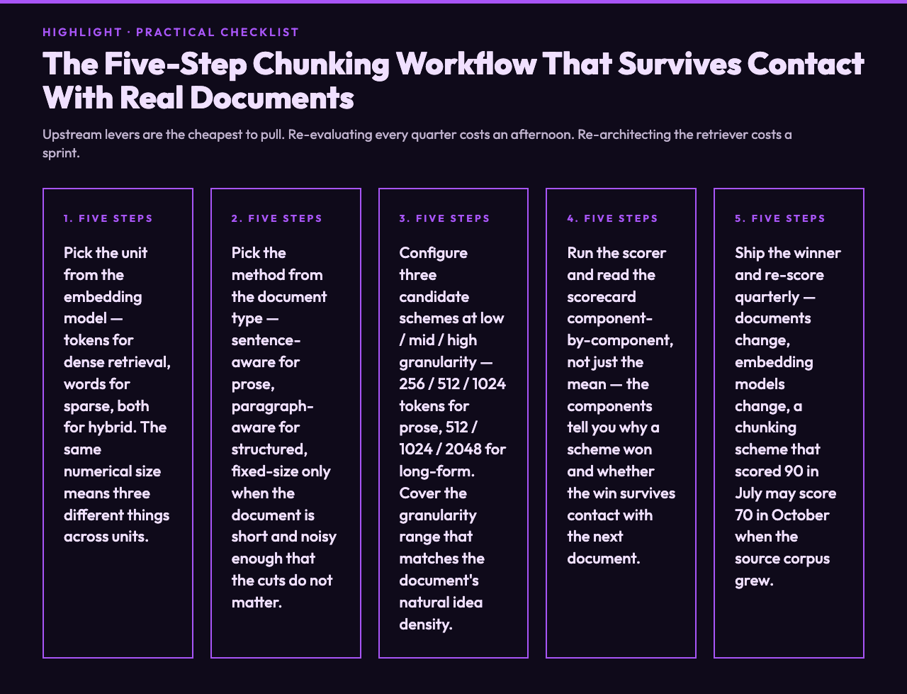
The five-step chunking workflow that survives contact with real documents
Putting the pieces together: a chunking workflow that turns the three decisions and four metrics into a reproducible loop.
- Pick the unit from the embedding model — tokens for dense retrieval, words for sparse, both for hybrid.
- Pick the method from the document type — sentence-aware for prose, paragraph-aware for structured documents, fixed-size only when the document is short and noisy enough that the cuts do not matter.
- Configure three candidate schemes at low / mid / high granularity (e.g. 256 / 512 / 1024 tokens for prose). Cover the granularity range that makes sense for the document’s natural idea density.
- Run the scorer on the document. Read the scorecard component-by-component, not just the mean.
- Ship the winner and re-score quarterly. Documents change, embedding models change, and a chunking scheme that scored 90 in July may score 70 in October because the source corpus grew.
The reason the loop matters: chunking is the upstream lever, and upstream levers are the cheapest to pull. Re-evaluating every quarter costs an afternoon. Re-architecting the retriever because the chunks are too wide costs a sprint.
Where chunking ends and retrieval begins
Once the chunks are sized right, the retriever has a fighting chance. Embedding models encode each chunk as a single vector, cosine similarity ranks them against the query, the top-k go to the LLM. The retriever’s job is to surface chunks whose idea-density matches the query’s idea-density. That matching is impossible when the chunks are 4,000 tokens wide (the entire chapter) or 12 tokens narrow (one phrase). It works when the chunks are 256–512 tokens of one idea, with enough overlap that the boundary between two adjacent chunks does not lose the cross-reference.
The same scoring framework that picks chunking also picks the embedding model, the similarity threshold, and the re-ranker — but those are downstream decisions. Chunking is the one that decides whether the retriever is even being asked the right question. Get it right, and the rest of the pipeline has something to work with. Get it wrong, and no amount of re-ranking recovers the missing context.
The AI RAG Chunk Quality Scorer is built for this loop — paste a document, configure three schemes, get a scorecard, ship the winner. For teams building RAG on top of LangChain or LangChain samples, OpenAI embeddings and OpenAI API patterns, or a vector database like Chroma or Pinecone with reference vector database implementations, the scorer is the upstream check that makes the downstream choices defensible. Run it before you index, not after the support tickets start.