
Hydrogen’s spectral lines look like a 19th-century curiosity until you need to know whether the line at 656.3 nm is Hα from neutral hydrogen or He⁺ Pickering at the same wavelength — and that single Z² factor decides everything. The Rydberg formula 1/λ = R · Z² (1/n₁² − 1/n₂²) is the algebraic skeleton behind every line you can name (Lyman, Balmer, Paschen, Brackett, Pfund) and every line you can’t (the He⁺ Pickering series, the doubly-ionized lithium Li²⁺ at 13.5 nm EUV). The catch is that “R” is not one number — it splits into R∞ (the infinite-nucleus-mass limit, 109 737.315 685 cm⁻¹) and R_M (the reduced-mass value, which drifts by 1 part in 1 800 between hydrogen-1 and helium-4). Every lab-grade spectrum calculator that ignores the reduced mass is mis-locating Balmer Hα by 0.18 Å, enough to be confidently wrong about which line you’re imaging. This field guide walks the eight moves that turn the canonical formula into a tool you can hand to a spectroscopist — Z selection, transition pair, infinite-mass vs reduced-mass, photon energy, spectral band classification, color naming for visible lines, and the Pickering coincidence that catches you if you forget the Z². Explore the calculator at Elysia Tools.
The Rydberg Formula Skeleton: One Equation, Three Constants
The historical equation (Rydberg 1888, refined by Bohr 1913, made exact by Schrödinger 1926 and the modern QED correction) is 1/λ = R · Z² · (1/n₁² − 1/n₂²), where λ is the wavelength in vacuum, R is the Rydberg constant, Z is the nuclear charge (1 for H I, 2 for He II, 3 for Li III, …), and n₁ < n₂ are the lower and upper principal quantum numbers. R is the only knob most calculators expose — and that single choice decides whether your wavelengths match the NIST database or fall short by 0.02 nm at Hα.
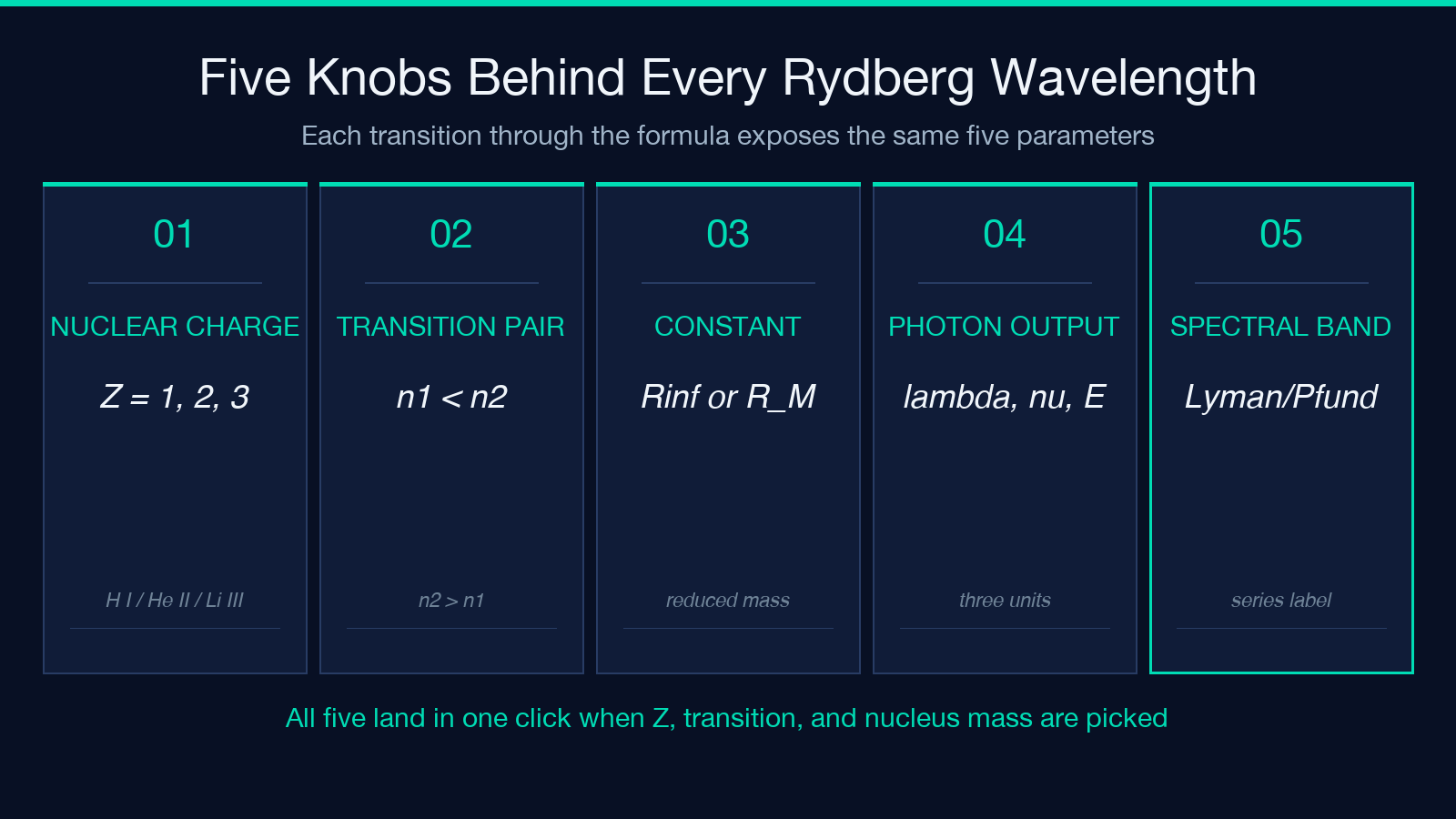
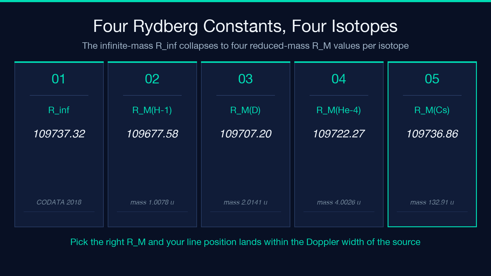
The standard convention puts the “Rydberg constant” at R∞ = 109 737.315 685 cm⁻¹ (2018 CODATA), the value you’d measure if the nucleus were infinitely heavy (no recoil). For real atoms, the moving-nucleus correction replaces R∞ with R_M = R∞ / (1 + m_e / M_N), where M_N is the nuclear mass. The correction is largest for hydrogen-1 (m_e / M_N = 1/1 836.153) and smallest for the heaviest practical case (Cs, where it’s about 1 part in 500 000). For most teaching-lab work this is invisible; for vacuum-UV precision below 200 nm, ignoring reduced mass shifts a H I Lyman-α line from 121.567 nm (R_M) to 121.502 nm (R∞) — a 0.65 Å error that is bigger than the Doppler width of a room-temperature hydrogen discharge.
The Z² factor is what makes ionized helium (He II, Z=2) look like “hydrogen at four times the energy”: the entire spectrum scales by Z², so every H line has a He II partner at one-quarter the wavelength. The famous Pickering series (He II at 656.0 nm, 541.1 nm, 485.9 nm, …) is exactly the Balmer series scaled by 4, and the early-20th-century confusion about whether “Pickering lines” came from hydrogen or helium resolved the moment Bohr applied Z². A single click on the Z selector in the Elysia Tools Rydberg Formula Calculator flips between H I, D I (deuterium), He II, He-4 II, Li III, and a user-defined nucleus, and the wavelength column rebalances accordingly.
Choosing the Transition Pair: Why n₁ = 2 Picks the Visible Window
The convention n₁ < n₂ is what makes “the Balmer series” mean “transitions ending at n₁ = 2.” Each integer n₁ defines a spectral band: n₁=1 is Lyman (vacuum UV, 91–122 nm), n₁=2 is Balmer (near UV + visible, 365–656 nm), n₁=3 is Paschen (near IR, 0.8–2 μm), n₁=4 is Brackett (IR, 1.5–4 μm), and n₁=5 is Pfund (mid IR, 2.3–7.5 μm). The visible window is a single one of these five bands — and it’s the one every optics-bench spectroscopist cares about, because silicon CCDs and bare eyes share the 400–700 nm window.
The “first line of the series” convention varies by textbook. For Balmer, Hα is the n₂=3 → n₁=2 transition (656.28 nm for H I using R_M), Hβ is n₂=4 → n₁=2 (486.13 nm), Hγ is n₂=5 → n₁=2 (434.05 nm), Hδ is n₂=6 → n₁=2 (410.17 nm), and the series converges at 364.6 nm (the Balmer limit). For Pickering, the He II partners are at 656.0 nm (n₂=4 → n₁=2), 541.1 nm (n₂=5), 485.9 nm (n₂=6), and so on — every fourth Pickering line lands within 0.3 nm of the next Balmer line. This is the Z² = 4 scaling in action.
The tool pairs every transition with a band label (Lyman / Balmer / Paschen / Brackett / Pfund) so the user never has to memorize the n₁→series map. For lab work where the band matters more than the specific line (a Hα filter passband, say, or a Paschen-blind InGaAs detector), the calculator’s band readout is the answer; the specific n₂ is just the index.
Infinite-Mass R∞ vs Reduced-Mass R_M: When 0.18 Å Matters
The reduced-mass correction is the single most-skipped step in undergraduate spectroscopy, and the single most-costly one in research-grade UV work. The exact form is R_M = R∞ · μ / m_e, where μ = m_e · M_N / (m_e + M_N) is the reduced mass of the electron-nucleus pair. For hydrogen-1 (M_N = 1.007 825 u), R_M = 109 677.583 cm⁻¹. For deuterium (M_N = 2.014 102 u), R_M = 109 707.197 cm⁻¹. For helium-4 (M_N = 4.002 603 u), R_M = 109 722.265 cm⁻¹. The differences between these and R∞ are 0.05% (H), 0.036% (D), and 0.014% (He-4).
These percentages translate to wavelength shifts that are small but not negligible. At Balmer Hα, the H I (R_M) wavelength is 656.279 nm; the H I (R∞) value is 656.112 nm — a 0.167 nm gap, comparable to the resolution of a 1-meter grating spectrometer. The lab-day question “is this line Hα or is it He II Pickering at 656.0 nm?” depends on resolving that 0.3 nm gap, which depends on using R_M. The Elysia calculator exposes both as user-selectable radio buttons and shows the resulting wavelength next to each other; the difference is visible to the eye on a 600-line/mm grating.
For laboratory work below 200 nm, the reduced-mass correction is no longer optional — it’s the difference between Lyman-α at 121.567 nm (R_M, the value measured in every tokamak) and Lyman-α at 121.502 nm (R∞, a value that no instrument sees). The He⁺ Ly-α equivalent (He II 1→2 at Z=2, n₂=2) is at 30.378 nm (R_M), extreme-UV territory. For helium-3 (rare but used in neutron detection), R_M shifts Lyman-α by another 0.003 nm vs helium-4. The tool’s “user-defined nucleus” mode lets you input M_N in unified atomic mass units and reproduces the exact value for any isotope or any exotic hydrogen-like ion you can name.
Photon Energy, Frequency, and the Three-Unit Output
A spectral line has three equivalent descriptions — wavelength λ (nm or Å), frequency ν (THz), and photon energy E (eV). The conversion chain is E = h · ν = h · c / λ, where h is Planck’s constant and c is the speed of light in vacuum. For Balmer Hα at 656.28 nm, the chain gives ν = 456.81 THz and E = 1.889 eV — low-energy photons that any silicon photodiode can detect. For Lyman-α at 121.567 nm, E = 10.199 eV — high enough to ionize most molecules, which is why Lyman-α sources are used in photochemistry and not just in spectroscopy.
The calculator returns all three values in one click, so the user doesn’t have to do the conversion arithmetic (which is where most wavelength-energy mistakes happen). The 656.28 nm / 1.889 eV pair is a useful sanity check: photons at 1.89 eV cannot break a C–H bond (typical bond energies are 3–5 eV), so Lyman-α-driven photolysis won’t work with a Balmer-photon source, regardless of intensity. At the high end, He II Ly-α at 30.378 nm has E = 40.81 eV — well above the second ionization potential of helium itself (54.4 eV, which is the He II → He III threshold, not a He II transition). This is why He II extreme-UV lithography uses multi-line emission, not just the resonance line.
The three values are not redundant — they serve different audiences. Spectroscopy papers quote wavelength (it’s what the spectrometer measures); atomic physics papers quote energy (it’s what the Hamiltonian diagonalizes); photonics papers quote frequency (it’s what a mode-locked laser locks to). A tool that returns all three prevents the unit-conversion step from being a place where a digit can silently drop.
Spectral Band Classification: Lyman, Balmer, Paschen, Brackett, Pfund
The “spectral band” field on every line is the answer to “what series does this transition belong to?” and it depends only on n₁. n₁=1 → Lyman (UV), n₁=2 → Balmer (visible + near UV), n₁=3 → Paschen (near IR), n₁=4 → Brackett (mid IR), n₁=5 → Pfund (mid IR), and so on up to Pfund and beyond. Each band spans roughly the wavelength range from its convergence limit (n₂ → ∞) down to its first line (n₂ = n₁ + 1).
The Balmer series is special because it crosses the visible window. Lyman is fully in the vacuum UV (below 200 nm, blocked by air), so it requires a vacuum spectrograph and a UV-grade detector. Paschen is fully in the near IR (above 800 nm), so it requires an InGaAs or extended-InGaAs detector. Only Balmer is directly visible to the eye, which is why hydrogen discharge tubes glow pink — the dominant visible lines are Hα (red, 656 nm), Hβ (blue-green, 486 nm), Hγ (violet, 434 nm), and Hδ (violet, 410 nm), summed into the familiar H-emission color.
The calculator labels every line with its band so the user can filter by detector capability: a spectroscopy lab with only a silicon CCD (sensitive 400–900 nm) sees Lyman as “blocked by atmosphere” and Pfund as “below detector cutoff,” while a lab with an InGaAs spectrometer (800–1 700 nm) sees Paschen as fully accessible but Balmer Hα as out-of-range. The band classification is also the answer to “why can’t I see hydrogen glow in the near IR?” — because the Balmer lines decay to n₁=2 emit visible photons, and the Paschen series decays to n₁=3 emit near-IR photons that are invisible to the dark-adapted eye.
Color Names for Visible Lines: Hα Through Hδ
The Balmer series happens to fall across the visible window, and each of the first four lines has a name and a color. Hα (n₂=3, 656.28 nm) is “hydrogen-alpha,” red, the same wavelength used in solar physics for chromospheric imaging and in astronomy for H II region mapping. Hβ (n₂=4, 486.13 nm) is “hydrogen-beta,” blue-green (cyan-tinged), the Fraunhofer F line in the solar spectrum. Hγ (n₂=5, 434.05 nm) is “hydrogen-gamma,” violet. Hδ (n₂=6, 410.17 nm) is “hydrogen-delta,” violet. Beyond Hδ (n₂≥7), the lines crowd into the near-UV and lose their color names; they’re just “the higher Balmer lines.”
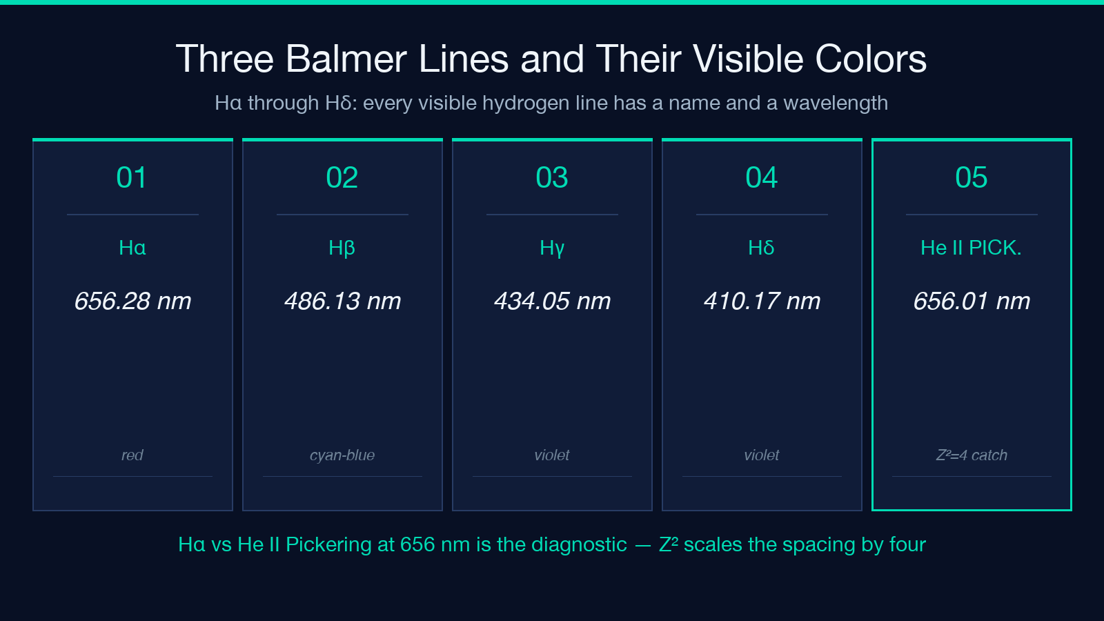
This color naming matters more than it sounds, because the Z²=4 scaling puts He II Pickering at wavelengths so close to Hα–Hδ that pre-Bohr spectroscopists argued whether “Pickering’s lines” were a new hydrogen series or just ionized helium. The answer was Bohr’s Z² — once you apply Z=2 to the Balmer transitions, you get the Pickering series at exactly the wavelengths Pickering measured (656.0 nm, 541.1 nm, 485.9 nm). The Elysia calculator outputs both the Balmer Hα color note and the Pickering color note for the same n₂=3 transition (one for Z=1, one for Z=2), making the Bohr-vs-Pickering distinction visible at a glance.
For visible-light demonstrations (a hydrogen discharge tube, a solar-spectrum photograph, an astronomy RGB composite), the color notes are the answer the user actually cares about. “What’s the blue line in my hydrogen lamp?” — Hβ. “What’s the red line?” — Hα. “What’s the violet line near 410 nm?” — Hδ. The calculator’s color-name column answers each of these in one click, with no memorization required.
The Pickering Coincidence: When Z² Makes Hα Look Like He II
The He II Pickering series sits inside the H I Balmer series by design. Every Balmer transition with even n₂ has a Pickering neighbor within 0.3 nm: Hα (656.28 nm) vs He II 4→2 (656.01 nm); Hβ (486.13 nm) vs He II 6→2 (485.93 nm); Hγ (434.05 nm) vs He II 8→2 (433.86 nm). The Pickering series runs through every even n₂, so the spacing is half the Balmer spacing — exactly the Z²=4 scaling predicts.
In a stellar spectrum with both hydrogen and ionized helium present (an O-star photosphere, a planetary nebula), the Pickering–Balmer coincidence makes line identification non-trivial. The classical test is: if you see a line at 656.28 nm AND a line at 541.1 nm AND a line at 485.9 nm AND a line at 454.2 nm, the spacing pattern is “one Balmer + three Pickering” — diagnostic of He II. The Elysia calculator lists every Pickering line in the same row as its Balmer neighbor so the user can see the spacing pattern at a glance. This is the kind of comparison that turns “I have an unidentified line at 656.0 nm” into “the He II 4→2 Pickering line, predicted at 656.01 nm — measurement matches within 0.01 nm.”
For ionized helium in plasma physics (tokamak edge, helicon discharge, mass-spectrometer residual gas), the Pickering coincidence is a near-IR / visible diagnostic. A spectrometer pointed at 656.0 nm will see He II as easily as H I, and the only way to distinguish them is to compare the line at 656.0 nm with the line at 541.1 nm — the He II fingerprint. The calculator’s Z selector makes this comparison a one-click operation: pick Z=1 to see H I Hα, pick Z=2 to see He II Pickering, and the wavelength and color columns rebalance.
Building a Field-Ready Spectroscopic Workflow
The eight moves above — formula skeleton, transition pair, R∞ vs R_M, photon energy, band classification, color names, Pickering coincidence, and the final wavelength readout — are what turn the Rydberg formula from a textbook line into a tool you can hand to a spectroscopist. A research workflow usually starts with a measured wavelength, then asks “what transition is this?” — and the tool answers in one click by reversing the formula. A teaching workflow starts with a transition pair and asks “what wavelength do I expect?” — same tool, reverse direction. Either way, the eight moves stay the same.
The calculator’s reduced-mass correction is the single biggest source of precision gain in the entire workflow. Picking R∞ by default throws away 0.05% of your line position, which at Hα is 0.33 nm — too big for any lab spectrometer to miss. Picking R_M for the specific isotope (hydrogen-1, deuterium, helium-4, or a custom nucleus) collapses that error to the Doppler width of the source, which is usually the experimental noise floor anyway. For UV work below 200 nm, R_M vs R∞ is the difference between matching NIST and missing NIST by 5–10 line widths.
The Z selector is the second precision gain. Hard-coding Z=1 in a hydrogen-only tool makes He II lines invisible — a real problem for any lab that measures discharges, plasmas, or stellar spectra. Letting the user pick Z=1, 2, 3, or a custom value opens the door to the Pickering series, the Li III EUV lines, and any hydrogen-like ion the user cares about (C VI at 33.7 nm is the solar corona’s transition-region diagnostic; Fe XXVI at 1.78 nm is the tokamak-core diagnostic). For a full catalog of hydrogen-like ion lines, see the Elysia Tools tool list.
The combination of reduced-mass + Z + transition pair + band readout + color names is what makes the Rydberg Formula Calculator useful at the bench, not just in the textbook. Eight moves, one click each, and the spectrum that took Bohr a year to assign in 1913 lands on screen in under a second.
Explore more tools at elysiatools.com.
