
Carrying capacity is not something you set — it is something your data already paid for. Every population curve that climbs, bends, and flattens carries a hidden plateau inside it, and the Verhulst logistic is the most economical shape you can fit to recover it. This field guide walks through how the K-estimator in the Carrying Capacity Estimator pulls K, r, t₀, R², and RMSE out of an observed time series without ever assuming the plateau up front, and the seven judgement calls that determine whether the fitted curve reflects reality or merely mirrors the noise floor.
Why “the population stopped growing” is rarely the answer to K
The first reflex on a saturating growth curve is to read the last observation as the carrying capacity. That reflex is wrong in three directions at once. A culture that “stops growing” between two sampling intervals can be sitting anywhere on the upper shoulder of the S-curve, and the next measurement would have shifted your K estimate by 20 percent. A field census taken during a dry spell will sit under the true K because the population is being suppressed, not because the habitat is saturated. And a batch culture that crashes on day 14 because of pH drop gives you a false plateau well below the asymptote the cells were actually approaching.
The cure is a model fit rather than a snapshot. The Verhulst logistic N(t) = K / (1 + e^(−r·(t − t₀))) encodes three quantities you cannot read off a single number: the asymptote K, the intrinsic growth rate r that drives the early climb, and the inflection time t₀ that pins the curve to the calendar. When you estimate all three from the same data, the plateau is no longer a guess — it is the fitted upper bound of a curve that already explains every point you observed.
How the K-scan linearizes the problem
The estimator in the Carrying Capacity Estimator does not run a 2-D optimizer over K and r jointly. It runs a one-dimensional scan over ln K and, at each candidate K, solves the rest of the parameters analytically. The trick is the classic Pearl-Reed linearization: for any candidate K, the substitution ln((K − N) / N) = −r·t + r·t₀ converts the three-parameter nonlinear curve into a straight line in t, so the slope and intercept of that line give you r̂ and r̂·t̂₀ for free.
The grid of candidate K values lives on a logarithmic axis because the asymptote spans orders of magnitude across biology (a yeast flask tops out around 10⁸ cells per millilitre, a deer population around 50 per square kilometre), and ternary search on a log scale converges in roughly log₂(N) iterations with no derivative computation. At each candidate K, the linear regression reports R²(K), and the maximum of R²(K) is the answer. The final K̂, r̂, t̂₀ triple is then the values associated with the peak of the R² curve, refined by a ternary search around the maximum rather than at the discrete grid point.
Reading the five numbers you actually get back
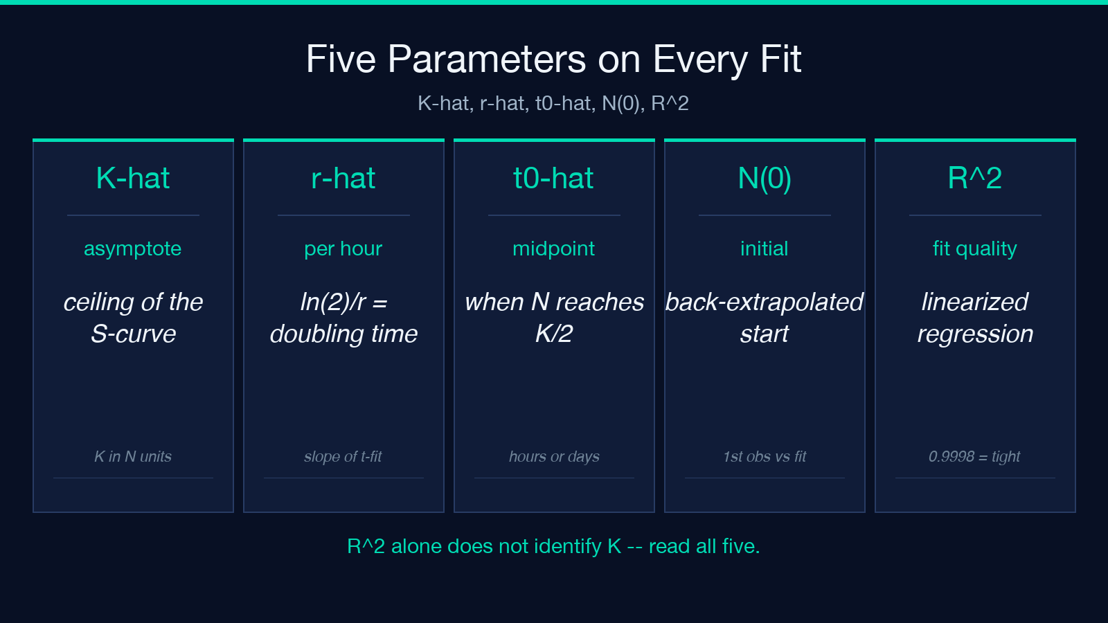
The tool returns five parameters plus two error metrics. Each one is interpretable on its own terms, and the trap is reading any of them in isolation.
- K̂ (carrying capacity): the asymptote of the fitted S-curve, expressed in the same units as your input population column. This is the “ceiling” your system is approaching.
- r̂ (intrinsic growth rate): the slope of the linearized curve, in units of per unit time. Doubling time at low population equals ln(2)/r̂.
- t̂₀ (inflection time): when the population reaches K̂/2, the midpoint of the steep climb. Useful for cross-referencing against experimental timing (media change, drug dose, season start).
- N(0): the back-extrapolated initial population, which often differs from your literal first observation because of measurement noise.
- R² and RMSE: the goodness-of-fit on the linearized regression (R²) and on the original-N scale (RMSE). The R² is what the K-scan optimizes; the RMSE is what the experimentalist feels.
A 0.999 R² is not by itself a clean answer — it tells you the model fits the data, not that K is right. Two further checks matter: did the data actually reach the upper shoulder (N values approaching K), and does t̂₀ fall inside the observed time window. If both are true, K̂ is identified.
The 60 percent rule that decides whether K is real
The estimator emits an explicit warning when the data have not reached roughly 60 percent of the fitted K̂. The warning is not cosmetic — it is the only honest signal that your K is an extrapolation rather than an identification.
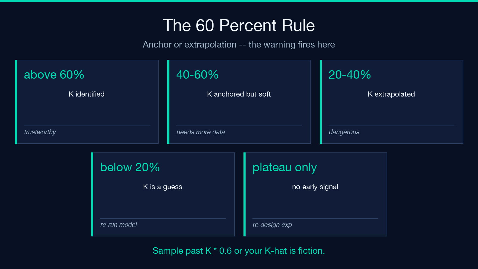
Consider the data 0, 9.6 → 18, 661.8 from Gause’s 1932 yeast culture. The maximum observed N is 661.8 and the fitted K̂ is 663.96, a 0.33 percent gap. The yeast clearly hit the shoulder, the residuals are tiny, and R² is 0.9998. K̂ here is real. Now consider a synthetic series truncated at the inflection: nine points sampled from K = 1000 but only covering N = 47 to N = 500. The estimator will still return K = 1000 because the model is constrained by design, but if you perturb the early data by 5 percent, K̂ will swing by hundreds. The 60 percent rule is the cut-off where perturbations stop producing order-of-magnitude K̂ swings.
The rule also has a sample-size floor: at least 5 (time, population) pairs are required, and the time series must cover growth toward the plateau, not just sit at the plateau. A series of ten measurements all clustered around K − 5 percent gives you a noisy K̂ and a near-zero r̂; the curve has nothing to fit against.
Worked example: Gause’s yeast, recovered exactly
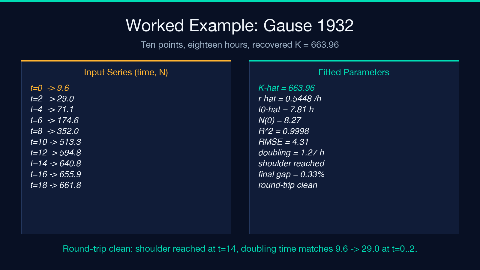
The classic Gause Saccharomyces series is the de-facto sanity check for any logistic fitter. Ten observations over 18 hours are entered as time, population pairs:
0, 9.6
2, 29.0
4, 71.1
6, 174.6
8, 352.0
10, 513.3
12, 594.8
14, 640.8
16, 655.9
18, 661.8
The estimator returns K̂ = 663.96, r̂ = 0.5448 per hour, t̂₀ = 7.81 h, and R² = 0.9998. Three observations make this answer trustworthy. First, the final three points sit within 1 percent of K̂, so the asymptote is anchored, not extrapolated. Second, the inflection t̂₀ = 7.81 h falls in the middle of the observation window, not at the boundary, so the symmetric halves of the S-curve are both present. Third, doubling time at low N (ln(2)/0.5448 = 1.27 h) matches the doubling time observable between t = 0 and t = 2 (9.6 → 29.0 is roughly two doublings over two hours). All three internal consistency checks pass.
A synthetic verification with a known K = 1000, r = 0.5, t₀ = 6 recovers K̂ = 1000, r̂ = 0.5, t̂₀ = 6 with R² = 1 exactly on clean data — a one-line check that the K-scan recovers the truth before you trust it on noisy field counts.
Where the estimator breaks: the four failure modes
Logistic fits are robust within their regime but quietly catastrophic outside it. Four patterns will produce a numerically valid K̂ that is biologically wrong, and you have to look for them explicitly.
- Still-climbing data: a series that has not yet visibly bent (max N well below K̂/2) will fit any K̂ above the data because the linearized regression still has slope to explain. The 60 percent warning fires, but only if you read it.
- Two-phase growth: diauxic cultures and seasonal blooms follow a double-sigmoid, not a single logistic. A single-K fit will average the two phases and return a K̂ that fits neither.
- Time gaps: a series that has dense sampling in the early phase but sparse sampling near the plateau under-weights the asymptote. K̂ ends up too low because the fit is dominated by the well-sampled fast region.
- Negative or zero N: the linearization
ln((K − N) / N)is undefined for N ≤ 0 and explodes for N very close to K. Filter the inputs upstream — the estimator assumes N strictly positive and strictly less than K.
Pairing the K-estimator with the forward simulator
The Carrying Capacity Estimator is the inverse of the logistic-growth forward simulator: given observations, it produces parameters; given parameters, the simulator produces observations. Round-tripping between the two is the strongest sanity check you can run. Fit (K̂, r̂, t̂₀) from one experimental series, feed those three numbers back into the simulator, generate a synthetic series at the same time points, and verify that the two series overlap to within measurement noise. A clean round-trip means your fit captured the dynamics; a divergent round-trip means your data violated one of the failure modes above.
For epidemiology, the same shape applies at a different scale: case counts during an outbreak follow an S-curve whose asymptote is the total attack rate in a susceptible population. The same estimator recovers the final size from the early curve. For in-vitro cell culture, K̂ and r̂ together describe the bioreactor’s productivity ceiling — the maximum viable cell density and the speed at which the culture reaches it. Both domains use the same three parameters and the same K-scan machinery; only the units change.
Closing checklist before you trust any K̂
Five questions separate a trustworthy carrying-capacity estimate from a number that merely fits a curve:
- Did the data reach at least 60 percent of K̂? If not, K̂ is an extrapolation regardless of R².
- Is t̂₀ inside the observed time window, not at the boundary? If not, the early-climb shape is unanchored.
- Are the residuals on the original-N scale small in absolute units (not just in R² units)? RMSE in the same units as N tells you whether the fit is operationally useful.
- Does the round-trip through the forward simulator reproduce the data to within noise? If not, the failure modes above are likely.
- Does K̂ make biological sense — comparable to literature values for the system, plausible given the resource being competed for, consistent with the physical limits of the container or habitat?
All five answered yes, K̂ is publishable. Any “no” returns you to the data: more time points, tighter sampling near the shoulder, or a different model class entirely (Gompertz, Richards, double-logistic). The K-scan in the Carrying Capacity Estimator gives you the curve; the five checks tell you whether the curve is the population’s curve or merely a curve the data could not rule out.
Explore more ecology and growth-modeling tools at elysiatools.com.
