
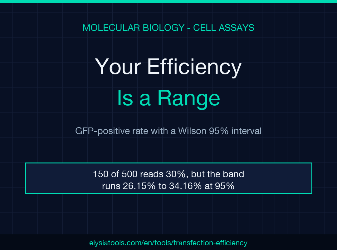
A transfection efficiency is not a measurement. It is a range wearing a percentage sign. You count 150 GFP-positive cells out of 500, write 30% in the notebook, and move on — but the honest answer is 26.15% to 34.16%, an eight-point band that swallows most of the differences the next optimization experiment tries to detect.
Each percentage on your plate hides a margin you did not write down
A cell count is about as binomial as biology gets. Each cell sits above your GFP threshold or below it, so a proportion built from those counts carries sampling error that shrinks only as the count grows. The lab notebook records the point estimate and throws away the distribution behind it.
There is a second reason the margin goes missing: the textbook interval is the wrong one at small counts. The normal approximation, p ± 1.96 × sqrt(p(1−p)/n), needs enough cells for the sampling distribution to look symmetric. At low efficiency it misbehaves, and at exactly zero positive cells it collapses to a zero-width interval, which proves nothing about a condition you have barely sampled. The Wilson score interval inverts the hypothesis test instead of approximating around the observed proportion, so it stays inside 0 and 100 and stays sensible when the count is small. Wilson published it in 1927; Newcombe’s 1998 study measured the alternatives and found the score form the safest at small n. The transfection efficiency calculator uses that form and returns the interval beside the percentage in single-measurement mode, which is the only reason I trust a two-digit efficiency with a single well behind it.
The 8-point band inside 150 out of 500
Put the numbers on the bench. 150 GFP-positive cells among 500 means p = 0.300, and the Wilson interval runs 26.15% to 34.16%. The width is 8.01 percentage points.
That width breaks experiments. Bump the count to 170 out of 500 and the point estimate is 34.00%, with an interval of 29.98% to 38.26%. A different reagent that genuinely produces 34% is indistinguishable from the 30% control, and a reviewer who asks for the number alone cannot see that. The tool prints both.
The interval is not decoration, and it is not a hedge. It is the resolution of the instrument you used, and it belongs in the same sentence as the result.
Why 50 cells and 2,000 cells tell different stories
Hold the efficiency constant at 30% and vary only how long you count. Here is the ladder:
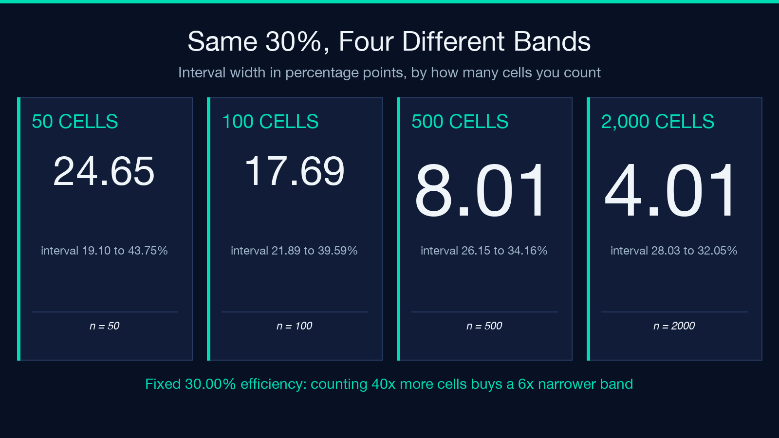
- 15 of 50 cells: 30.00%, interval 19.10% to 43.75%, width 24.65 points
- 30 of 100 cells: 30.00%, interval 21.89% to 39.59%, width 17.69 points
- 150 of 500 cells: 30.00%, interval 26.15% to 34.16%, width 8.01 points
- 600 of 2,000 cells: 30.00%, interval 28.03% to 32.05%, width 4.01 points
The pattern is the square-root law, and it sets your bench economics. Going from 50 cells to 500 costs tenfold the clicking and cuts the band to a third of its width. Going from 500 to 2,000 costs four times the clicking and reduces the band by only half. If you are choosing between conditions, the count that makes two conditions separable is usually 500 per condition, not 50. And if you counted 50 because the field looked crowded, you did not measure a 30% transfection, you measured “somewhere between 19% and 44%” — stopping early does not fix the problem, it hides it.
Three wells are not a triplicate
Single-mode intervals describe counting noise. They say nothing about well-to-well variation, which includes plating density, reagent mixing, and the fact that one corner of the plate always seems colder. Replicate mode is where the tool earns its place in a lab notebook. Feed it parallel counts and it returns per-well efficiencies, the mean, and the sample standard deviation.
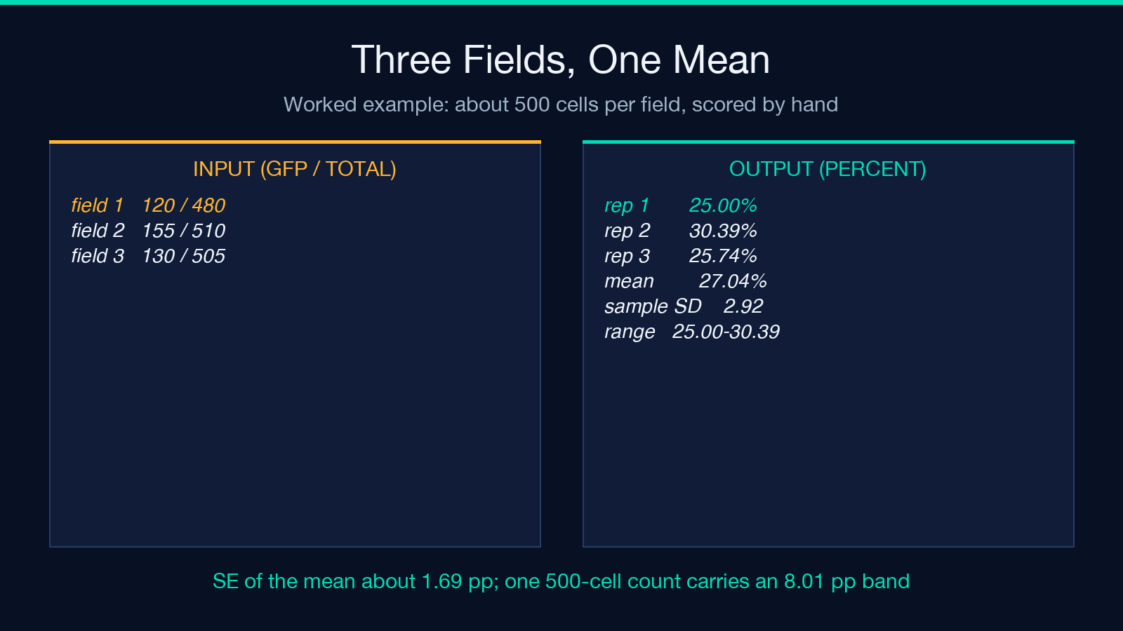
Here is the tool’s own worked example. Three microscopy fields scored 120 of 480, 155 of 510, and 130 of 505 cells. Those are 25.00%, 30.39%, and 25.74%. The mean is 27.04% with a sample SD of 2.92 points and a range of 25.00% to 30.39%.
Two observations, and they point in opposite directions. The mean of a genuine triplicate is a far better estimate than any single well: three wells of roughly 500 cells give a standard error near 1.69 points, so the mean carries a band of about 3.4 points, less than half the 8 points a single 500-cell count carries. For instance, halving that count to 250 cells per well widens the mean’s band again, so the third well buys precision you cannot get by counting longer in one place. But look at the spread between the wells themselves: 5.4 points separate the best field from the worst, and the worst case here is 25.00% against a mean of 27.04%. That spread is your realistic noise floor, and it is larger than the effect most optimization experiments claim to find.
An honest gap: according to the output’s own model line, the SD uses an n−1 denominator, and a three-replicate SD is itself a rough estimate. With three wells you hold two degrees of freedom, so the SD you print could plausibly be half or double the true spread. Treat 2.92 as an order of magnitude, not a constant.
Pooled or averaged: the two-tenths decision nobody records
Two defensible ways to combine replicate counts exist, and most notebooks do not say which one was used. Pool all cells and divide: 405 of 1,495 is 27.09%. Average the replicate percentages: 27.04%. The gap is 0.05 points, and at similar well sizes it never matters.
It matters when the well sizes differ. Take two wells — 100 of 200 and 400 of 2,000. The ratios are 50.00% and 20.00%, so the mean of ratios is 35.00% while the pooled ratio is 22.73%. That is a 12.27-point disagreement produced entirely by the choice of denominator. Pooling increases the influence of the largest well; averaging gives each well equal weight.
The calculator computes the mean of ratios, and the model line in its output says so. If a collaborator’s spreadsheet pools instead, expect the numbers to diverge the moment well sizes drift apart — which they do whenever one field is easier to count than another.
The band edges do not respect your thresholds
The tool sorts results into bands: excellent at 70% and above, good from 30% to 70%, moderate from 10% to 30%, low below 10%. The bands are useful shorthand. They are also point estimates, and at the boundary the label can be wrong in a way the number is not.
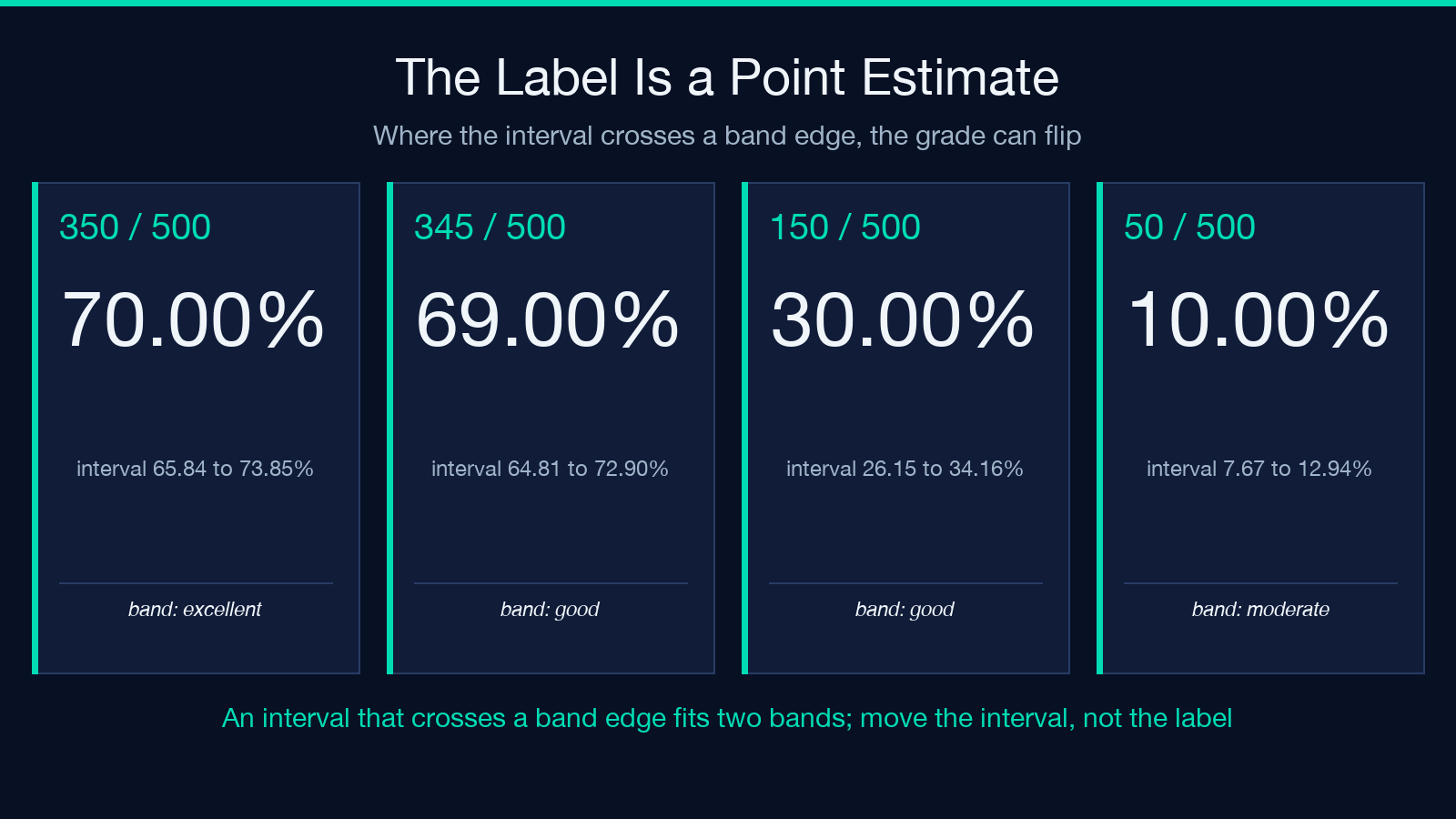
Score 350 of 500 and the tool returns the label “excellent” at 70.00%. The interval is 65.84% to 73.85%, so the same data is compatible with a good-grade transfection and with an excellent one. Score 345 of 500 and the label flips to good at 69.00%, yet the interval top reaches 72.90%. On the lower boundary, 150 of 500 reads good at 30.00% while its interval dips to 26.15%, squarely inside moderate.
A reagent swap that improves the mean from 68% to 71% and one that improves it from 71% to 74% look like different outcomes on the label, and neither is distinguishable from noise at n=500. So design the comparison around the interval, not the band: aim to shift the whole range. For example, a change that moves the lower bound from 26.15% to 31.00% has done more work than a change that pushes the point estimate up two points.
Gate the dead cells before you score the living ones
Three assumptions sit under these numbers, and the tool states them in its output instead of hiding them. Dead and detached cells must be gated out before scoring. One GFP threshold must apply to all cells. Transient expression must be read at its 24-to-72 hour peak.
The first assumption carries the most weight. A dead cell can scatter into the fluorescent channel, and a stress response can shut the plasmid down entirely, so an ungated count mixes uptake efficiency with toxicity and calls the sum “transfection.” Pair the score with a viability read — the trypan blue viability calculator turns a hemocytometer differential count into a percentage — and if you count by hand instead of with a cytometer, the hemocytometer cell counter gives you the cells-per-milliliter denominator the count depends on. A 30% transfection at 95% viability and a 30% transfection at 65% viability are not the same experiment, even though they print the same number.
Measure the noise floor before you change the protocol
The cheapest experiment in transfection optimization is the one nobody runs: dose the same plasmid into three wells, count all three, and compute the spread. That number costs one plate and one afternoon, and it converts future comparisons from a guess into a test you can design against — a benchmark to hold each new condition to. If the spread you measured is 2.92 points, a condition that shifts the mean by two points has not changed anything you can see. If it shifts the mean by eight, you have found something.
Two practical notes from the numbers: First, ask for at least four replicates before quoting an SD, because at n=2 the sample SD is barely defined and the tool returns null for a single replicate instead of inventing one. Second, keep the raw counts in the record alongside the percentages, since the percentage alone cannot be re-analysed and the counts can. Clarify which convention you used — pooled or averaged — because a reviewer will assume the other one. Explore the full calculator and its related lab tools at elysiatools.com.
I began this piece believing the problem was precision: that we report 30% where we should report 30.00%. The point is the opposite. We report a point where the data supports an interval, then spend a week of bench time chasing differences smaller than the interval we never printed. Print the band, compare the band, and the next experiment finally means something.
本文有中文版:你的转染效率是一个区间,不是一个数
