The Math Behind Every Song You’ve Ever Streamed Is Made of Circles
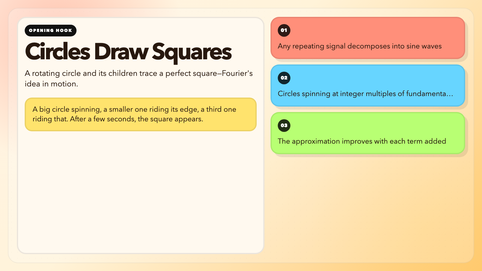
You draw a square on a screen. Then a tool starts drawing it back—but with rotating circles. A big circle spinning, a smaller one riding its edge, a third one riding that. Three different speeds. Three different radii. After a few seconds, the square appears. Perfect. Built from nothing but rotation.
This is the Fourier series. It is also why your music files are small, your photos compress without disappearing, and your phone can make a call at all.
The Audacious Claim That Took 15 Years to Publish
In 1807, Joseph Fourier submitted a paper to the French Academy of Sciences claiming that any repeating signal can be written as an infinite sum of sine and cosine waves.
Lagrange objected. The academy rejected the paper. Fourier waited. Published a book in 1822. The idea eventually won.
The math works like this: a square wave’s coefficients follow a clean pattern—1/n for odd harmonics, zero for even ones. One circle, one-third circle, one-fifth circle, one-seventh circle. The circles shrink proportionally. Add infinitely many and you get the square.
The catch is Gibbs phenomenon. At every sharp corner, the approximation overshoots by about 9%. Mathematicians did not fully understand why until 1906—nearly a century later. You can make the overshoot narrower in time. You cannot make it disappear.

Fourier stumbled on this while modeling heat diffusion through metal rods. He needed better math for differential equations. He accidentally invented the foundation of digital signal processing.
What the Visualization Actually Shows
The Fourier Series tool turns the formula into motion.
Choose a square wave. The animation shows circles spinning at integer multiples of the fundamental frequency. The largest circle is the fundamental. Each subsequent circle is half the radius of the previous odd term. With 5 circles, the reconstruction is crude. With 20, it is close. With 100, you cannot see the difference.
You can draw any closed shape by hand. The tool decomposes your curve using a Discrete Fourier Transform and rebuilds it live from spinning circles. The reversibility gets me every time—any shape in, circles out, circles back into the shape. Engineers call this a transform precisely because it is an exact translation between two equivalent descriptions of the same signal.
Two Domains, One Signal
Every signal has two simultaneous representations.
In the time domain, you see the raw waveform—voltage on a wire, air pressure from a speaker, pixel brightness across a photo. In the frequency domain, you see which frequencies are present and how strong each one is.
A piano playing middle C produces energy at 261 Hz, 522 Hz, 783 Hz, and higher multiples. A flute playing the same note produces a different mix of those same frequencies. Your ear does an automatic frequency analysis, which is why you recognize your friend’s voice through a heavily compressed phone call—the frequency balance survives even when some detail does not.
The Convolution visualization shows what happens when two signals interact. Blur an image in Photoshop: the blur kernel convolves with the photo. Add reverb in Pro Tools: the room’s impulse response convolves with the dry sound. The convolution theorem says this operation in the time domain is equivalent to multiplication in the frequency domain. Without this equivalence, every reverb plugin would be orders of magnitude slower.
The Number That Made CDs Possible
How many measurements do you need to capture a signal perfectly? The Nyquist-Shannon theorem says: at least twice the highest frequency you want.
Human hearing maxes out around 20 kHz. Twice that is 40 kHz. CDs were standardized at 44.1 kHz, which leaves engineering margin for imperfect anti-aliasing filters. The theorem was proposed by Nyquist in 1928, formalized by Shannon in 1949, and adopted for audio CDs in 1982. It has not changed since.
The Sampling Theorem visualization demonstrates what happens when you violate the rule. Sample a high-frequency wave below Nyquist and it reappears as a completely different frequency. Wagon wheels spinning backward in films. Moiré patterns in digital photos. Aliasing artifacts.
Where It Lives in Your Phone
MP3 was standardized in 1993 by the Fraunhofer Institute in Germany. The format uses a modified DCT to decompose audio into frequency bands, then applies a psychoacoustic model—based on Fourier analysis—to discard frequency components masked by louder nearby ones. A typical 128 kbps MP3 discards about 90% of the raw audio data. In double-blind listening tests conducted by the RIAA and others, most subjects cannot reliably distinguish 128 kbps MP3 from CD audio. Most cannot reliably distinguish 192 kbps.
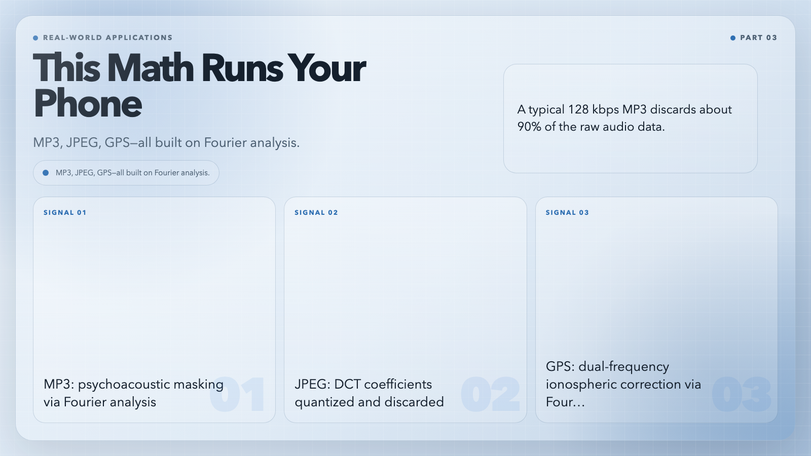
JPEG, standardized in 1992 by the Joint Photographic Experts Group, applies the same principle in two dimensions. Each 8×8 pixel block is decomposed into 64 DCT coefficients. JPEG quantizes away the high-frequency coefficients, then run-length encodes the result. A 24-megapixel raw photo at 72 MB compresses to a 2–3 MB JPEG with visually lossless quality.
GPS satellites transmit on L1 (1575.42 MHz) and L2 (1227.60 MHz). Dual-frequency GPS receivers measure differential dispersion across the two bands to correct ionospheric delay—this correction is a Fourier technique. Without it, GPS accuracy degrades from sub-meter to tens of meters. The atomic clocks on GPS satellites maintain time to within 8 nanoseconds per day, using Fourier-based phase-lock loops.
The Question Nobody Has Answered Yet
Gibbs phenomenon is mathematically unavoidable. The 9% overshoot at discontinuities cannot be designed away. This is not a technical limitation you can fix with better hardware—it is a fundamental property of approximating discontinuous functions with smooth ones. It shows up in JPEG artifacts at high compression ratios. It shows up in digital audio at steep filter edges.
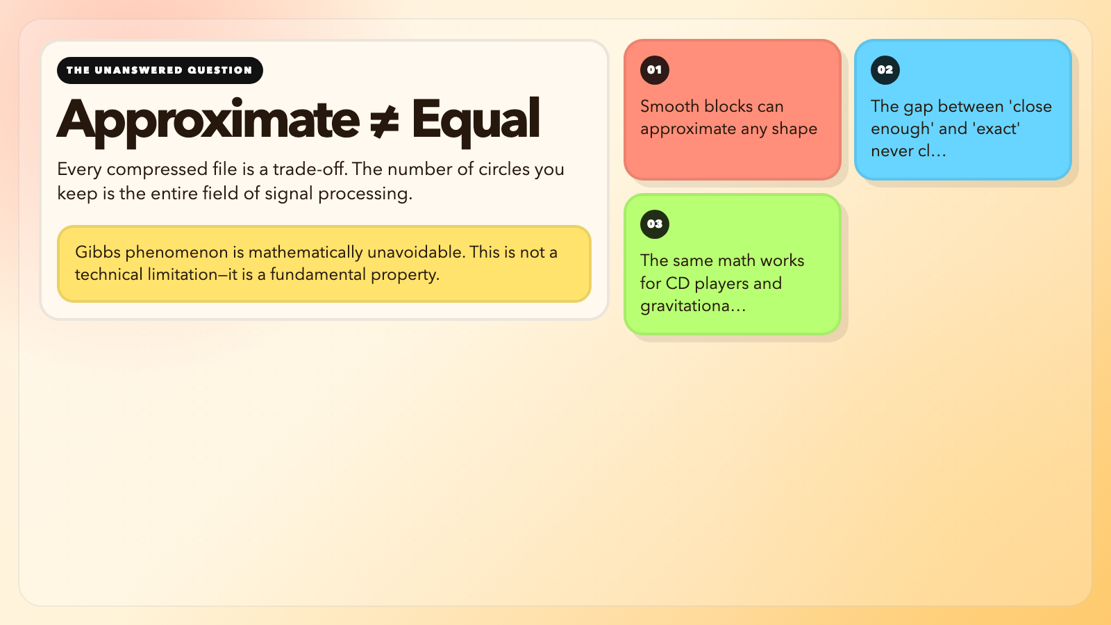
Fourier showed smooth building blocks can approximate anything. But approximation and equality are different things. Every time you compress a file, you are choosing how many circles to keep. That choice is signal processing, and it always involves a trade-off between accuracy and cost.
The Fourier Series visualization hands you that trade-off directly. Draw a shape, watch it come apart into spinning circles, and ask yourself: how many do you actually need? The answer changes depending on whether you are designing a CD player or detecting gravitational waves. It is the same math.