# 6 Free Interactive Physics Visualizations That Make Invisible Forces Finally Make Sense
In 2015, LIGO detected two black holes colliding 1.3 billion light-years away. The signal lasted 0.2 seconds. The displacement it measured? Less than one-thousandth the diameter of a proton.
The scientists who built LIGO described it as hearing the universe for the first time. That metaphor undersells how strange the detection actually was.
These six free visualizations let you see what LIGO was listening for — and four other phenomena where the underlying mechanism stays invisible until you build intuition for the dynamics.
—
Gravitational Waves — See What LIGO Actually Measured
A gravitational wave ripples spacetime itself when two massive objects orbit each other. LIGO’s detector bounces laser light between mirrors 4 km apart — the wave stretches one arm and compresses the other by a fraction of a proton’s width, changing the light’s travel time by about 10⁻¹⁸ seconds.
The Gravitational Waves visualization simulates this. Watch two black holes orbit and radiate waves outward in concentric rings. Adjust mass, orbital radius, and rotation speed — watch the wave amplitude change in real time.
The pattern that emerges: faster orbits and stronger fields produce more energetic waves. As the merger approaches in the simulation, the orbital frequency increases — exactly matching LIGO’s first observed signal, known as GW150914.
Link: https://elysiatools.com/en/visualizations/gravitational-waves
—
Beat Frequency — When Two Sounds Collide and Create a Third
Play two sine waves at 440 Hz and 443 Hz simultaneously. Your ear doesn’t hear two tones. It hears one tone pulsing 3 times per second — that’s the beat frequency, equal to the difference between the two source frequencies.
This isn’t a trick of perception. The two waves physically interfere, adding and subtracting at each point in time. The result is a wave with the average frequency (441.5 Hz) modulated by the difference frequency (3 Hz).
The Beat Frequency visualization uses the Web Audio API to generate real audio. Set one frequency, set another, and watch the combined waveform. The math is wave interference, and the visualization makes it audible and visible simultaneously.
The applications reach far beyond music: spectrometers detect gas composition by measuring beat frequencies, GPS receivers correct signal errors the same way, and neurons in the inner ear use this principle to detect frequency differences in sound.
Link: https://elysiatools.com/en/visualizations/beat-frequency
—
Coriolis Force — Why Hurricanes Spin Different Directions
The Coriolis force isn’t a real force. It’s an apparent deflection that appears when describing motion from a rotating reference frame. Earth rotates eastward at roughly 1,670 km/h at the equator, tapering to zero at the poles. That rotation deflects winds to the right in the Northern Hemisphere, left in the Southern.
Fire a projectile from any latitude in the Coriolis Force visualization and watch it curve. The same initial velocity produces different trajectories depending on where you start. The visualization also models the Foucault pendulum, atmospheric circulation cells, and cyclones — showing why hurricane rotation is opposite in the two hemispheres.
The counterintuitive part: Coriolis deflection is strongest at the poles, zero at the equator. Weather systems near the equator behave differently not because it’s hot, but because the rotational effect hasn’t built up yet.
Link: https://elysiatools.com/en/visualizations/coriolis-force
—
Lissajous Figures — Drawing With Sound
Connect two oscillators to an XY plotter — one driving horizontal motion, one vertical — and you get Lissajous figures. The shape is entirely determined by the frequency ratio and phase difference. A 1:1 ratio at 0 degrees gives a diagonal line. A 1:2 ratio produces a parabola. A 1:1 ratio at 90 degrees produces a perfect circle.
The Lissajous Figures visualization lets you set frequency ratios from 1:1 to 1:5 (and beyond) and adjust phase offsets continuously. Watch the figure morph as you cross clean integer ratios — those are the ratios where the figure closes and repeats. Non-integer ratios never quite close, filling in the plane over time.
Engineers used Lissajous figures to test whether two AC power sources were synchronized — if the figure was stable and stationary, the frequencies matched exactly. If it drifted, they knew something was off. Today the same principle appears in oscilloscope calibration and musical synthesis.
Link: https://elysiatools.com/en/visualizations/lissajous-figures
—
Stern-Gerlach Experiment — Where Quantum Mechanics Gets Real
In 1922, Otto Stern and Walther Gerlach fired silver atoms through a magnetic field gradient. Classical physics predicted a continuous smear of deflection — atoms should land everywhere depending on their orientation. The atoms landed in exactly two discrete spots.
Two. Not a range. Two.
This was the first direct evidence of quantum spin, the property that makes electrons behave like tiny bar magnets with only two allowed orientations: up or down.
The Stern-Gerlach Experiment visualization simulates the apparatus. Fire atoms through the field and watch them split into two beams. Then stack a second magnet rotated 90 degrees and fire one of the resulting beams through it — it splits again, into two more beams. This is quantum measurement in its most concrete form: not uncertainty about the result, but discrete outcomes that cannot be predicted from classical physics.
The visualization’s value is in making the discrete-vs-continuous distinction viscerally clear. Classically, you expect a smear. Quantum mechanically, you get two points. The simulation doesn’t let you unsee it.
Link: https://elysiatools.com/en/visualizations/stern-gerlach-experiment
—
The Intuition Worth Building
These phenomena have something in common: they describe dynamics of things you can’t see directly. Gravitational waves distort spacetime itself. Beat frequency is wave interference in real audio. Coriolis deflection only appears when you calculate from a rotating frame. Quantum spin has no classical analog at all.
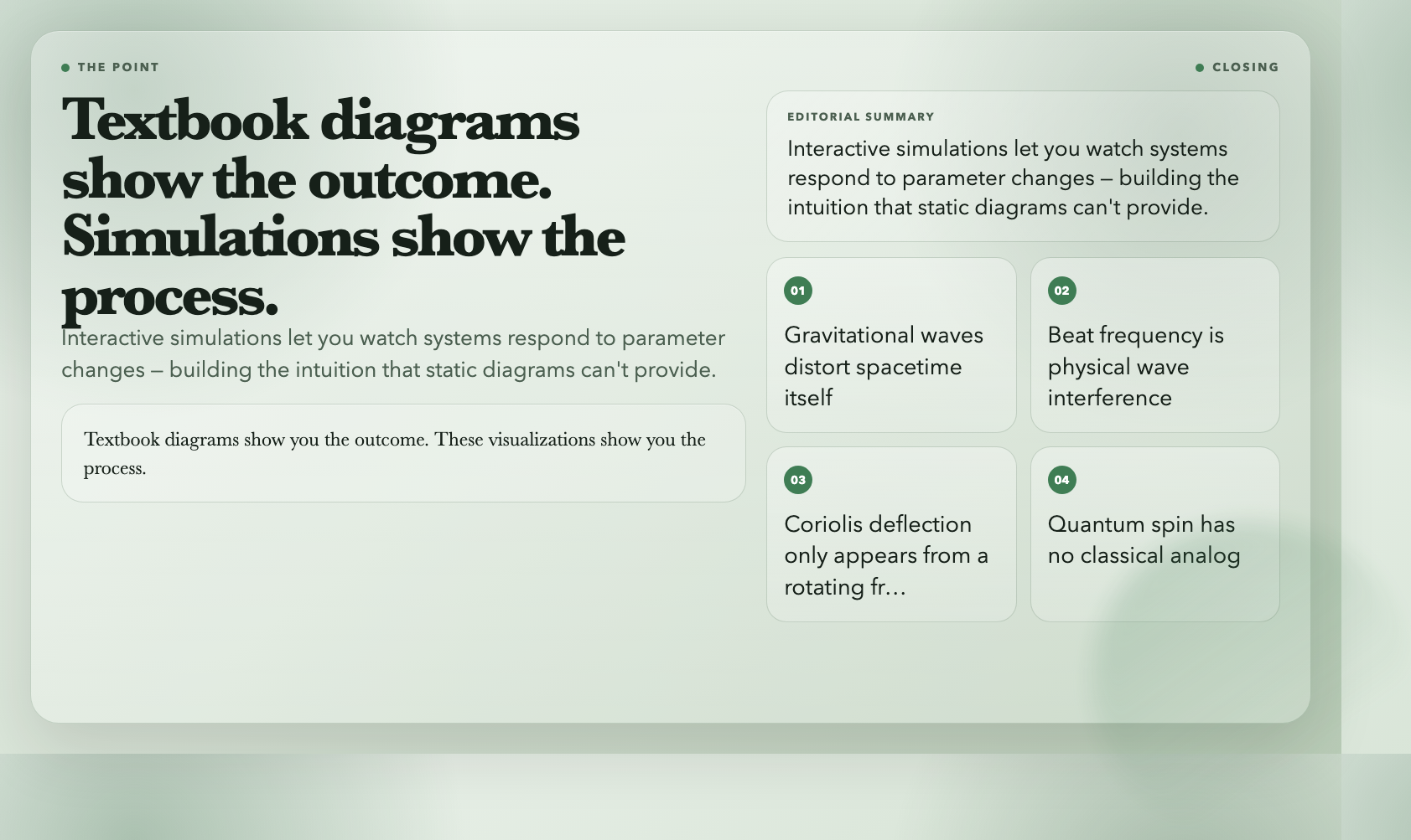
Textbook diagrams show you the outcome. These visualizations show you the process — how something changes when a parameter changes, what the full trajectory looks like, why the result is what it is.
The gravitational wave from LIGO was a 0.2-second chirp. The Stern-Gerlach experiment split atoms into two discrete spots 100 years ago. The Coriolis force shapes every hurricane on Earth. None of these are intuitive until you see the dynamics — and you can only build that intuition by watching the system respond to changes.
That’s what interactive simulations are for.
*All 6 visualizations are free at elysiatools.com/en/visualizations.*