Why the Simplest Pendulum You Can Build Is Also Impossible to Predict
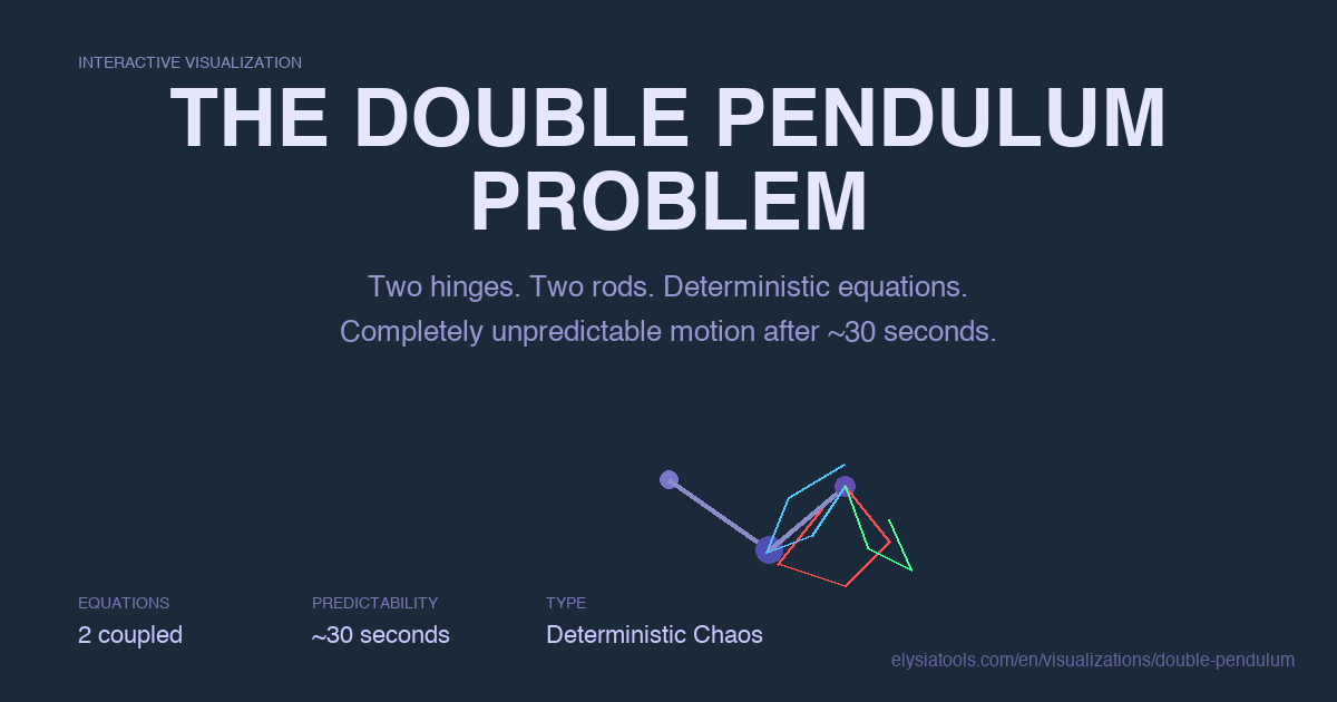
Drop a ball off a cliff. You can calculate exactly where it’ll be in 10 seconds. Push a double pendulum — two rods attached end to end — and after 30 seconds you might as well be watching a coin flip.
The double pendulum is one of the most elegant demonstrations in all of classical mechanics. It’s just two hinges, two rods, gravity, and math. Yet it produces motion that no equation can predict beyond a few seconds. This isn’t a flaw in your calculator. It’s a fundamental feature of the universe.
The Setup Takes 30 Seconds
A regular pendulum is simple. Lift it to an angle, let go, and it swings back and forth in a predictable arc. The math was worked out by Galileo in the 1600s. You can write its motion in a single clean equation.
Now attach a second pendulum to the end of the first. You’ve added one more link, one more mass, one more angle to keep track of. The equations that describe its motion don’t fit on a napkin anymore. Two coupled differential equations, each one feeding into the other through trigonometric functions. Change one angle by a fraction of a degree, and both equations spit out a completely different answer.
That’s the key. The system is nonlinear. Small changes don’t produce proportionally small effects. They produce entirely different effects.
Launch Three of Them and Watch the Universe Glitch
There’s a demo built into the ElysiaTools Double Pendulum simulator that makes this visceral: the butterfly effect button.
It launches three double pendulums. Each one starts at nearly the same angle. The difference between the first and second is 0.001 radians — about 0.057 degrees. The difference between the second and third is another 0.001 radians. You can barely distinguish the starting positions with your eye.
For the first few seconds, all three move identically. The trails they leave on the screen overlap almost perfectly.
Then, somewhere between 10 and 20 seconds, they diverge. The first trail starts to drift left. The second goes right. The third loops wildly in a different direction. Three systems, started with microscopic differences, now look completely unrelated.
Lagrangian Mechanics: Where the Math Gets Beautiful
Classical mechanics can be written in two equivalent ways. Newton’s approach — force equals mass times acceleration — works fine for the double pendulum, but the equations get tangled. You have to track forces at every hinge, in every direction, at every moment.
Lagrange’s approach is different. Instead of forces, you think in terms of energy and constraints. You define the system’s kinetic energy T and potential energy V, then write a single function called the Lagrangian: L = T − V. Apply the Euler-Lagrange equations, and the constraints fall away. What emerges are the equations of motion in their cleanest form.
For the double pendulum, those equations involve both angles (θ₁ and θ₂) and their angular velocities (ω₁ and ω₂). They’re coupled — the acceleration of the first pendulum depends on the position of the second, and vice versa. The coupling happens through sine and cosine functions, which are themselves nonlinear. That’s where the chaos lives.
The equations, for those who want them:
θ̈₁ = [m₂l₁ω₁²sinΔθ cosΔθ + m₂g sinθ₂ cosΔθ + m₂l₂ω₂²sinΔθ − (m₁+m₂)g sinθ₁] / [l₁(m₁+m₂) − m₂l₁cos²Δθ]
>
θ̈₂ = [−m₂l₂ω₂²sinΔθ cosΔθ + (m₁+m₂)(g sinθ₁ cosΔθ − l₁ω₁²sinΔθ − g sinθ₂)] / [l₂(m₁+m₂) − m₂l₂cos²Δθ]
where Δθ = θ₁ − θ₂.
What matters isn’t the algebra. What matters is that these equations are deterministic — given the same starting conditions, they always produce the same motion — yet the motion is unpredictable beyond a short time window. This combination has a name: deterministic chaos.
What Chaos Actually Means
The word “chaos” in physics doesn’t mean random. It means deterministically unpredictable. The system follows exact rules. But those rules have a structural property: tiny differences in where you start get amplified exponentially.
With a regular pendulum, if you start at 45 degrees instead of 44.9 degrees, the period changes by about 0.1%. The error stays bounded.
With a double pendulum, that same 0.1-degree difference doesn’t just change the period slightly. It changes the entire future trajectory. The error doesn’t stay bounded — it grows. After enough time, the prediction error is as large as the system itself.
This is what people mean when they talk about the butterfly effect: not that a butterfly in Brazil causes a tornado in Texas, but that the atmosphere is a system with the same mathematical structure as a double pendulum. Small uncertainties — like the flapping of wings — grow into large uncertainties — like weather patterns. You can’t predict weather three weeks out not because your computer is weak, but because the math itself won’t allow it.
The Phase Space: Seeing the Invisible
The double pendulum simulator includes a phase space view. Phase space is a way of visualizing a dynamical system beyond its physical motion. Instead of plotting positions in physical space, you plot one variable against its rate of change — in this case, θ₁ against ω₁, or θ₂ against ω₂.
For a regular pendulum, its phase space portrait is a simple oval. The system traces the same oval over and over, forever. Periodic. Predictable. Boring.
For a double pendulum, the phase space portrait is intricate and never quite repeats. As the system moves, it traces a path that fills the available space but never crosses itself (without damping). The shape it traces is called a strange attractor — a region in phase space that the system stays within, but never visits in exactly the same way twice.
You can watch this happen in real time on the ElysiaTools phase space visualization, which lets you switch between the physical simulation and the phase space view while the system runs.
Deterministic Chaos: Henri Poincaré’s Discovery
The mathematics of chaos was discovered almost by accident.
In the late 1800s, the French mathematician Henri Poincaré was working on the three-body problem — predicting the motion of three gravitationally interacting bodies, like the Sun, Earth, and Moon. He tried to find an exact solution. Instead, he found that the equations were sensitive to initial conditions in a way that made long-term prediction fundamentally impossible.
He didn’t call it chaos. That word came later. But he described exactly the phenomenon you’d see in a double pendulum simulation: tiny measurement errors growing until predictions become meaningless.
The full appreciation of chaos in the scientific community took until the 1960s and 1970s, when computers became powerful enough to actually iterate these equations and watch the sensitivity happen in real time. Edward Lorenz’s weather simulation in 1961 — where he discovered that rounding a number from 0.506127 to 0.506 produced completely different weather patterns — is the canonical story. But Lorenz was really rediscovering what Poincaré had found with a double pendulum’s worth of mathematics 80 years earlier.
Why You Should Care
Because chaos is everywhere.
The double pendulum is a model for real physical systems that behave the same way: coupled oscillators in mechanical engineering, certain chemical reactions, plasma physics, and biological rhythms. The same mathematical structure that makes the double pendulum unpredictable shows up in the heartbeat, in the electrical activity of neurons, in the timing of epidemics.
It’s also a useful test bed for understanding what predictability means. If a mechanical system with just two moving parts can’t be predicted beyond a minute or so, what does that say about economic models, climate projections, or neural networks?
The honest answer is: it says these systems are hard. Not impossible — but hard in a specific, mathematical way that requires honest acknowledgment of uncertainty rather than false precision.
Try It Yourself
The Double Pendulum simulator on ElysiaTools is free to use. A few things worth trying:
- Start with the Horizontal preset. Both pendulums start at 90 degrees. Watch how the system transitions from regular swinging to wild spinning.
- Switch to the Butterfly Effect demo. Launch the three nearly-identical systems and watch how quickly they diverge.
- Add some Damping — drag the damping slider up to 0.1 or higher. With damping, the system eventually settles into a predictable periodic motion. This is the key difference: chaos requires energy input to stay chaotic. Take away the energy, and the system calms down.
- Watch the Phase Space tab while the simulation runs. You’ll see the strange attractor form in real time — the path filling space without ever quite repeating.
The double pendulum is one of the best tools in existence for building genuine intuition about chaos. No math background required. Just watch the trails diverge.