The Equation That Shows Why Simple Rules Create Infinite Complexity

There is a formula so simple that you can write it on a napkin:

x_{n+1} = r · x_n · (1 – x_n)

Three symbols. One multiplication. One subtraction. No randomness, no dice rolls, no quantum effects. It is called the logistic map, and for over a century it was studied as a model for animal population growth — the kind of equation that appears in introductory biology textbooks.

Then in the 1970s, mathematicians started feeding it to computers and discovered something that shattered centuries of mathematical intuition: this equation doesn’t just settle into predictable patterns. Under the right conditions, it generates chaos. True chaos. The kind where the future is determined by the past but still impossible to forecast.

The Diagram That Shows Order Becoming Chaos

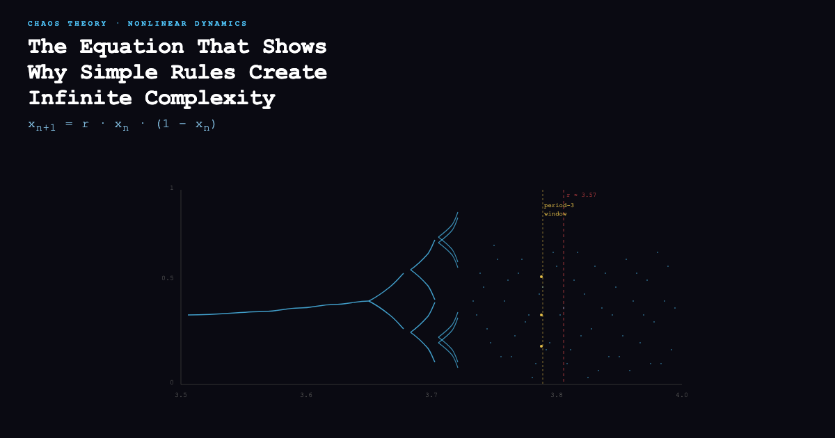
The bifurcation diagram is the clearest picture of this transition. On the horizontal axis is the parameter r — a single number you can dial from 3.5 to 4.0. On the vertical axis is x, the population value the system settles into after running for a while.

At low values of r, the diagram shows a single line. The system settles to one stable value. You know exactly where it ends up.

Then at r ≈ 3.0, something remarkable happens. The line splits. The system now oscillates between two values — population goes up, then down, then up again, forever. Period-doubling has begun.

Keep increasing r. At 3.449, two becomes four. At 3.544, four becomes eight. At 3.564, eight becomes sixteen. Each bifurcation happens faster than the last, compressed toward a critical threshold.

Then at r ≈ 3.56995, the branching stops making sense. The single line dissolves into a smear of points — infinitely many of them, packed together so densely they look like ink. The system has entered chaos.

This is not noise. This is not randomness. Every single point is generated by the same deterministic formula. The equation never varies. Only the value of r changes.

The Universal Constant Hidden in the Forks

Here is the part that made physicists and mathematicians genuinely excited. Mitchell Feigenbaum was studying these bifurcation diagrams in the mid-1970s when he noticed something peculiar. The gaps between successive bifurcations shrink by the same ratio each time, no matter what system you’re looking at.

He calculated that ratio: approximately 4.669201609…

This number — now called the Feigenbaum constant, or δ — appears everywhere period-doubling occurs. It is found in the logistic map, in electronic circuits, in fluid turbulence, in dripping faucets, in heart rhythm patterns, in population models, and in chemical reactions. The same number, again and again, in systems that have nothing to do with each other.

This is what physicists mean when they say a phenomenon is universal. The details of the system don’t matter. What matters is that it undergoes period-doubling. And if it does, it will obey Feigenbaum’s constants.

There is a second constant, α ≈ 2.502907, which describes how the bifurcation branches scale in width. Together, δ and α are to chaos what π is to circles — a fundamental property of the geometry of the transition itself.

The Windows Within Chaos

One of the most counterintuitive features of the bifurcation diagram appears after you enter the chaotic region. If you keep your eyes on the diagram rather than looking away, you will see something unexpected: clear, stable islands floating inside the chaos.

At r ≈ 3.83, the chaos briefly clears. A three-cycle emerges — the system visits exactly three values in a repeating pattern before chaos resumes. At r ≈ 3.74, there is a five-cycle. At r ≈ 3.905, a six-cycle.

These are not anomalies. They are called periodic windows, and their existence inside chaos is one of the most striking features of the logistic map. It means that even deep inside deterministic chaos, order is hiding — waiting to emerge when r takes on specific values.

This is the deep structure of nonlinear systems: chaos is not pure randomness. It contains pockets of stability. It contains self-similarity — zoom into any bifurcation region and you will see the same pattern that appears at the macro scale. The diagram is a fractal. Every magnification reveals the same architecture.

Why This Is Not Just a Mathematical Curiosity

The logistic map is deceptively simple, but its behavior is not anomalous. It is representative. The same period-doubling route to chaos appears in:

– Lasers: as you increase the pumping power, laser output transitions from steady to period-doubled to chaotic
– Cardiac rhythms: the transition from normal heartbeat to certain arrhythmias follows the same bifurcation pattern
– Climate systems: the onset of El Niño events and other climate transitions show period-doubling signatures
– Fluid dynamics: the transition from laminar to turbulent flow in pipes

The logistic map does not model these specific phenomena. But it captures their mathematical skeleton. The bifurcation diagram is, in a precise sense, the fingerprint of a system approaching chaos through period-doubling — and once you know what to look for, you start seeing Feigenbaum’s constants everywhere.

The Deeper Point About Determinism

The most important thing the bifurcation diagram illustrates is not any particular constant or phenomenon. It is the relationship between determinism and predictability.

Before the 1970s, most scientists assumed these were the same thing. If an equation was deterministic — if it had no random terms — then it should be predictable. Chaos was considered a curiosity, something that only arose in complex, high-dimensional systems.

The logistic map demolished this assumption. It is one-dimensional. It is deterministic. It is utterly unpredictable past the chaos threshold. No matter how precisely you know the initial value x₀, if r is in the chaotic regime, you cannot forecast the system beyond a handful of iterations. Feigenbaum himself reportedly spent weeks hand-calculating bifurcation points on a calculator before a computer was available to plot the full diagram — and when he finally saw it, he said it looked like the skyline of a city seen from a plane at night.

Edward Lorenz, working on weather models at MIT, arrived at the same conclusion from a different direction. He had stumbled on the same phenomenon by accident in 1961 — a weather simulation run with rounded numbers produced completely different forecasts than the original. His work and Feigenbaum’s converged on the same truth from different fields: deterministic equations can produce behavior that is effectively random, even when no randomness is present.

This is not a paradox. It is a property of nonlinear systems. And the world is nonlinear at almost every scale that matters — chemistry, biology, climate, economics, fluid dynamics. Which means the bifurcation diagram is not an exotic case. It is closer to the norm than the exception.

See It for Yourself

The Bifurcation Diagram tool on ElysiaTools lets you explore this transition interactively. Drag the parameter r from 3.5 to 4.0 and watch the system change from stable, to period-doubling, to chaotic. Enable the Feigenbaum constant overlay to see where successive bifurcations converge. Zoom into any chaotic region and observe the periodic windows emerge.

What makes this worth your time is not just the math. It is the fact that the same cascade — stable point, then 2-cycle, then 4-cycle, then chaos — appears in laser physics, cardiac arrhythmias, El Niño cycles, and fluid turbulence. The diagram is a map to a universal transition. Once you have seen it, you will start recognizing the fingerprints of Feigenbaum’s constants in systems you thought were outside your domain.