The Pendulum That Proves You Can’t Predict the Future
In 1961, Edward Lorenz ran a weather simulation on a computer at MIT. Then he ran it again. The two simulations started from what he believed were identical initial conditions. Within a few simulated months, they had diverged into entirely different climates.
The difference was 0.000127 — a rounding error in the sixth decimal place. Lorenz had not discovered a bug. He’d discovered chaos.
The Pendulum That Should Be Boring
A double pendulum is two pendulums chained together. Each obeys classical mechanics. The equations come from Lagrange’s formulation — 18th century math, fully worked out. Every parameter is known. There is no randomness, no quantum effects.
It should be boring. Instead, it is the cleanest demonstration of chaotic dynamics in classical physics.
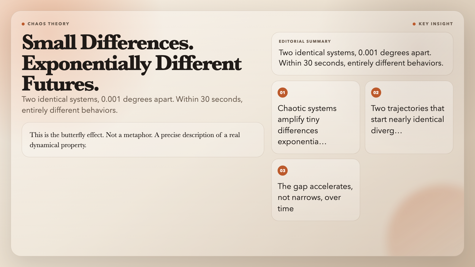
Small differences in starting conditions — 0.001 degrees between two copies — produce entirely different futures. Not gradually. Exponentially. The gap accelerates until the two trajectories have nothing to do with each other.
This is the butterfly effect. Not a metaphor. A precise description of a real dynamical property.
What It Looks Like
The Double Pendulum Chaos visualization on ElysiaTools shows this in real time.
Watch the second bob trace its path. It looks like calligraphy. Whorls, loops, sudden reversals, intricate patterns that never repeat. No two swings are alike.
Toggle multi-trail mode. The visualization runs several trajectories from nearly-identical starting points. They begin together, briefly overlap, then diverge. After 30 seconds, they might as well be running from different planets. The divergence is immediate and dramatic.
The phase space plot shows another chaos signature: the trajectory never closes. A periodic system loops back on itself. A chaotic system fills a region of space indefinitely without ever repeating.
The Equations
Two coupled second-order differential equations govern the system:
Equation 1:
(m₁ + m₂)L₁θ₁” + m₂L₂θ₂”cos(θ₁ – θ₂) + m₂L₂(θ₂’)²sin(θ₁ – θ₂) + (m₁ + m₂)gsinθ₁ = 0
Equation 2:
L₂θ₂” + L₁θ₁”cos(θ₁ – θ₂) – L₁(θ₁’)²sin(θ₁ – θ₂) + gsinθ₂ = 0
θ is angle. ω = θ’ is angular velocity. L is length, m is mass, g is gravitational acceleration. No randomness. Fully deterministic. These equations contain everything about the system’s future. And from them, chaos emerges.
How Scientists Found It Everywhere They Looked
Lorenz published “Deterministic Nonperiodic Flow” in the Journal of the Atmospheric Sciences (1963). Weather’s predictability horizon, he concluded, is roughly two weeks. Not because the physics is wrong, but because initial conditions cannot be measured precisely enough. The system amplifies errors faster than instruments can reduce them.
Robert May found it in ecology. In “Simple mathematical models with very complicated dynamics” (Nature, 1976), he showed that the logistic map — a single equation for population growth with density limits — produces chaos when its growth rate parameter r exceeds approximately 3.57. At r = 4, the output is statistically indistinguishable from random noise. Yet the equation is deterministic. May demolished the ecological consensus that populations naturally stabilize toward equilibrium.
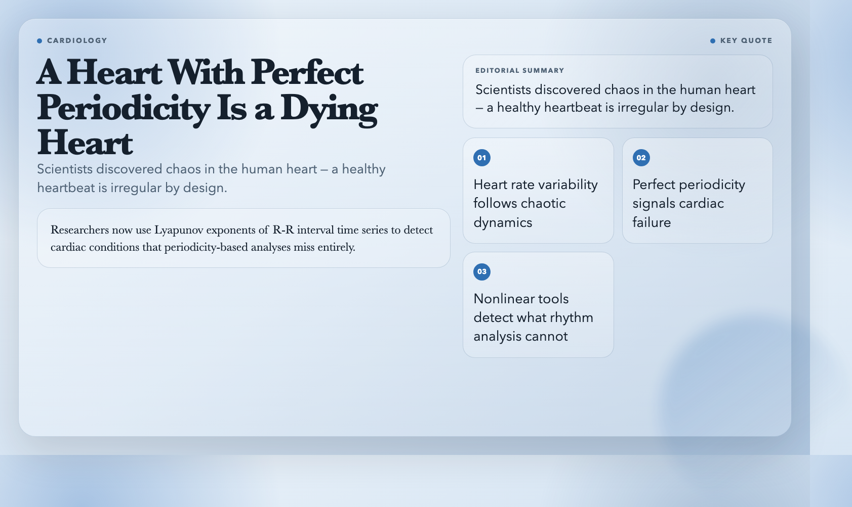
Cardiologists found it in the human heart. A healthy heartbeat varies in small, irregular ways reflecting feedback between the sinoatrial node, the autonomic nervous system, and blood pressure. A heart with perfect periodicity is a dying heart. Researchers now use Lyapunov exponents of R-R interval time series to detect cardiac conditions that periodicity-based analyses miss entirely.
Once scientists knew what to look for, they found chaos everywhere: fluid turbulence, bond trading, forest fire frequency, neural firing patterns, population cycles, power grids. The double pendulum was not an anomaly. It was a preview.
Why This Changes How You Should Think About Prediction
Most real-world systems that matter — economies, ecosystems, climate, social dynamics — are chaotic. Every model built from real data carries measurement error. In a chaotic system, that error compounds exponentially.
Climate models rest on sound physics. They are not guessing. Yet IPCC projections carry wide uncertainty bands because climate is chaotic. The difference between 1.5°C and 4°C of warming by 2100 partly comes down to whether the initial atmospheric state was measured to six decimal places or five. You cannot measure it precisely enough. You never will.
This does not make models useless. Short-term forecasts work. Understanding system structure is valuable. Knowing your system’s Lyapunov exponent tells you how far out predictions remain trustworthy. But long-horizon precision requires initial precision that is physically unattainable.
The Question the Pendulum Hands You
How much does the beginning determine the end?
For two rods, two masses, equations from 1788 — deterministic, energy-conserving — the beginning determines almost nothing. The system amplifies every microscopic difference until prediction becomes physically impossible.
Most complex systems operate the same way. Quietly. Deterministically. Past the horizon of anything you can calculate.
The difference is not whether you can predict them. You cannot. The difference is whether you design for that reality or pretend it isn’t there.
Run the Double Pendulum Chaos visualization on ElysiaTools. Watch the trajectories diverge. Then ask yourself what else is doing this, right now, without you noticing.