The Map That Shows Why the Same Starting Point Can Lead to Three Different Destinations

Start with a number on the complex plane. Apply a simple formula. Watch where it lands.

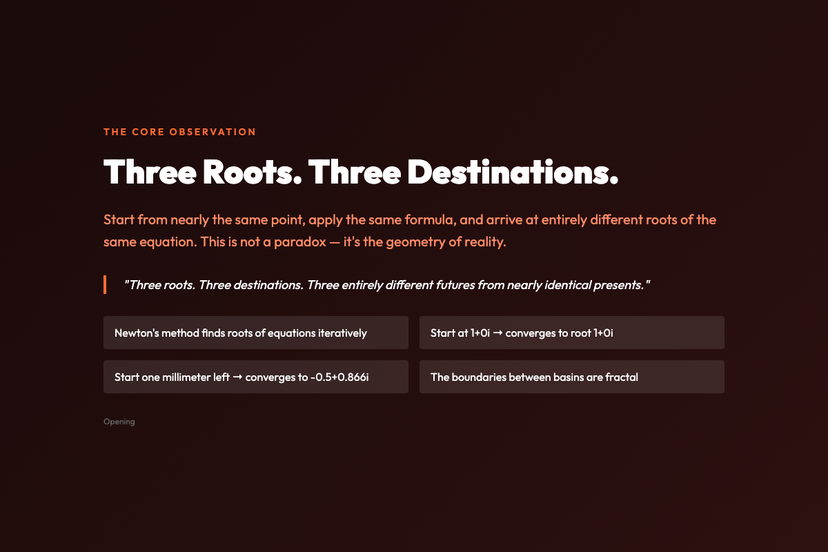
Now try again — but this time, start one thousandth of a millimeter to the left. If you’re using Newton’s method to find the cube roots of 1, your first attempt converges to 1 + 0i. Your second attempt — almost identical, impossibly close — converges instead to -0.5 + 0.866i. A third neighbor might send you to -0.5 – 0.866i.

Three roots. Three destinations. Three entirely different futures from nearly identical presents.

This isn’t a quirk. It’s the geometry of reality.

What Newton Fractals Actually Show

When mathematicians visualize the basins of attraction for Newton’s method applied to polynomial equations, they produce images of haunting beauty: vast regions of color, each hue representing a different root, separated by boundaries so intricate that no amount of zooming ever reveals a clean edge.

The image you’re looking at — generated by the Attractor Basin visualizer — shows this precisely. Every point on the plane is colored according to which root Newton’s method converges to when you start from that point. The boundaries between colored regions are not merely complex. They are fractal: self-similar at every scale, infinitely detailed, never quite resolving into simplicity no matter how far you zoom.

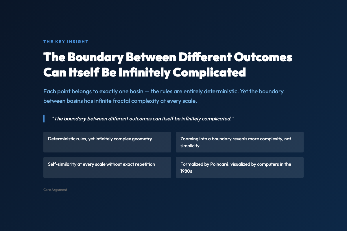
This is the counterintuitive core of the discovery that transformed how we understand dynamical systems: the boundary between different outcomes can itself be infinitely complicated.

A Brief History of Finding Roots

Newton’s method — the iterative technique for finding roots of equations — was formalized by Joseph-Louis Lagrange in the 18th century, though Isaac Newton described the underlying idea earlier. The method is straightforward: make a guess, find the tangent line at that guess, follow the tangent to the x-axis, use that point as your next guess, repeat.

For simple equations like x² – 4 = 0, this works beautifully. Start anywhere reasonable, and you’ll converge rapidly to ±2. The basins of attraction are clean, separate regions with straightforward boundaries.

But when Lagrange and later mathematicians applied the same technique to complex polynomials — equations with multiple roots in the complex number system — the clean picture fell apart.

Henri Poincaré, studying celestial mechanics in the 1880s, was among the first to recognize that simple iterative processes could produce outcomes so sensitive to initial conditions that they appeared random. His work on the three-body problem led him to understand that even deterministic systems could be fundamentally unpredictable in practice.

The full picture of Newton fractals — what they look like visually and what they mean mathematically — wasn’t clear until the 1980s, when computer graphics became powerful enough to render them. When mathematicians first saw these images on screen, the reaction was something close to disbelief.

The Fractal Boundary Problem

Here is the thing that makes Newton fractals philosophically unsettling, even now:

Each point in the complex plane belongs to exactly one basin. Every starting point has exactly one destination. The rules are deterministic, completely rigorous, entirely predictable in principle.

Yet the boundary between basins is infinitely complicated. Points that are arbitrarily close to each other — neighbors in the most literal geometric sense — can find themselves in entirely different basins, destined for entirely different futures.

This is not chaos in the colloquial sense. Newton’s method is not random. It is completely deterministic. But the structure of its basins creates a geometry that is, in a precise mathematical way, infinitely complex at every scale.

The mathematician Mitchell Feigenbaum, working in the 1970s on similar phenomena in logistic maps, discovered a related surprise: certain properties of these fractals are universal. The same fractal dimension appears at transition points across wildly different physical systems — from fluid turbulence to population dynamics to electronic circuits. The numbers that describe these transitions are constants, fixed points in the landscape of mathematical possibility.

What the Visualization Actually Shows

The Attractor Basin visualizer lets you explore this geometry directly. You can:

– Switch between different polynomial systems (Newton: z³ – 1, z⁴ – 1, z⁵ – 1, and custom variants, or quadratic maps like z² + c) – Watch trajectories trace their convergence in real time – Zoom into any region to see the self-similar boundary structure emerge – Adjust iteration limits and tolerance to see how the basins shift

The visualization makes one thing viscerally clear that equations alone cannot: the boundaries are not complicated in the way that a jagged coastline is complicated. They are complicated in a deeper, stranger way — a way that formal mathematical language describes but that only visual immersion truly conveys.

When you zoom into a boundary region, you don’t find simpler structures emerging. You find more of the same. The same patterns repeat at smaller scales, not perfectly identical but statistically self-similar. Zoom again. Same again. The complexity does not resolve; it multiplies.

Why This Matters Beyond Mathematics

The study of attractor basins and fractal boundaries turned out to be foundational to chaos theory. The same geometry that makes Newton fractals beautiful explains why weather is unpredictable beyond about ten days, why the double pendulum’s motion can never be precisely predicted, why the heartbeat sometimes settles into arrhythmia despite being driven by a perfectly regular pacemaker.

In each case, the system has multiple attractors — multiple possible steady states — and the boundaries between their basins of attraction are fractal. Initial conditions that seem nearly identical can find themselves on opposite sides of a boundary, leading to outcomes that diverge dramatically over time.

This is the deep connection: fractal basin boundaries are a geometric signature of sensitivity to initial conditions, and sensitivity to initial conditions is what makes long-term prediction impossible for a vast class of real-world systems.

Newton’s method, designed to find roots with maximum efficiency, thus became an unexpected portal into one of the most profound insights of 20th-century science: that simple rules can produce infinitely complex geometry, and that deterministic systems can exhibit behavior that is, in practice, indistinguishable from randomness.

Explore It Yourself

The Attractor Basin visualizer at ElysiaTools lets you generate your own Newton fractals and quadratic maps. Try the default z³ – 1 system first — three roots, three colors, three destinations from a single complex plane.

Then zoom into a boundary region. Pick a point in a blue area very close to a yellow boundary. Move one pixel. See where you land.

The geometry is waiting. It has no preference, no bias, no secret logic. It simply is — infinitely detailed, deterministically rigid, and strangely beautiful at every scale you choose to look.

Try it at ElysiaTools