The Simple Formula That Predicts Chaos

One equation. Four lines of Python. Infinite surprises.

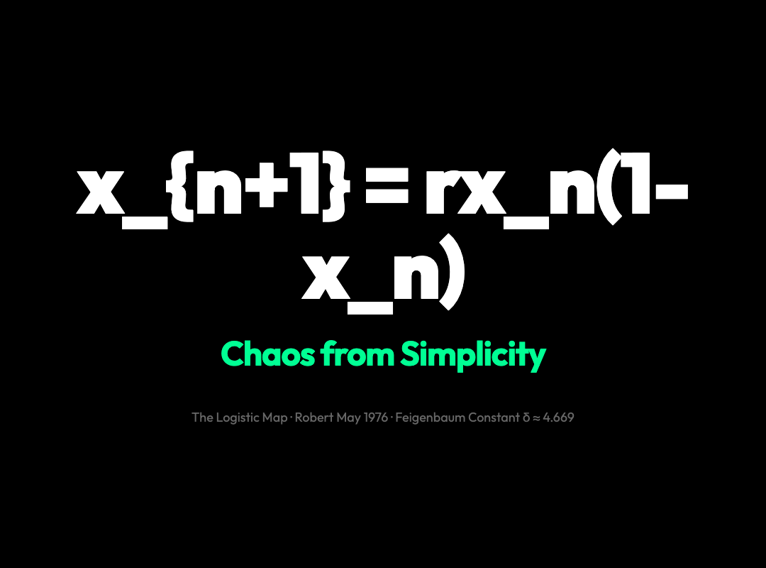
In 1976, biologist Robert May published a paper that would change how we think about prediction, complexity, and the gap between simplicity and chaos. The equation he studied looked almost too trivial to matter:

x_{n+1} = r · x_n · (1 − x_n)

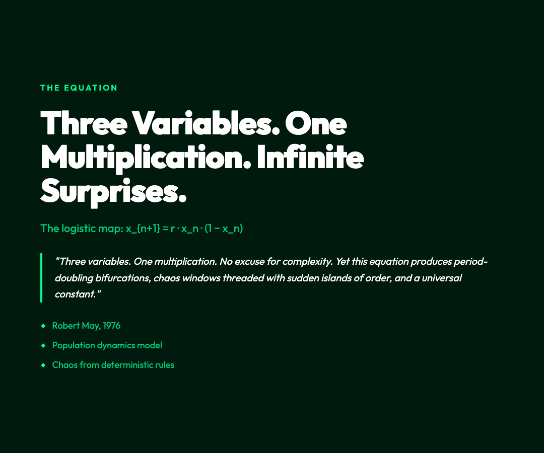
Three variables. One multiplication. No excuse for complexity.

Yet this equation — the logistic map — produces period-doubling bifurcations, chaos windows threaded with sudden islands of order, and a universal constant (δ ≈ 4.669) that appears in phenomena as distant as fluid turbulence and population collapse. It is the closest thing chaos theory has to a Rosetta Stone.

The Bifurcation Diagram: A Map of Everything

The clearest way to see what the logistic map does is to plot its long-term behavior across every value of r from 2.4 to 4.0. This is the bifurcation diagram — and if you haven’t seen it before, it looks like a river branching and branching again until it dissolves into structureless noise.

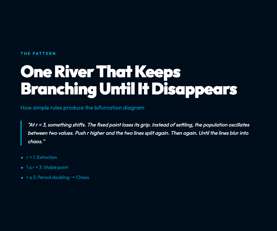
At r < 1, the system is already dead: x converges to 0 and stays there. Start at any population level and extinction is inevitable. The line is single and flat.

Between 1 and 3, the river runs to a single point — a stable fixed point. Whatever initial population you start with, it settles to the same equilibrium. Predictable. Boring. One line.

At r = 3, something shifts. The fixed point loses its grip. Instead of settling, the population oscillates between two values — a 2-cycle. The single river splits into two. This is the first bifurcation, and it happens at r ≈ 3.0.

Push r a little higher and the two lines split again at r ≈ 3.449. Now you have a 4-cycle: four population levels cycling in sequence. The branching accelerates. At r ≈ 3.544, it splits to 8. Then 16. Then 32.

At r ≈ 3.56995, the branching becomes so rapid that the lines blur into a continuous band. The system has entered chaos — not randomness, but deterministic chaos: perfectly governed by the equation, yet unpredictable in practice because tiny differences in initial conditions explode into wildly different outcomes.

The Feigenbaum Constant: Universality Hidden in the Pattern

As the bifurcation diagram reveals, the intervals between successive bifurcations shrink by a fixed ratio. Robert May and physicist Mitchell Feigenbaum independently discovered that this ratio converges to a constant:

δ ≈ 4.669201609

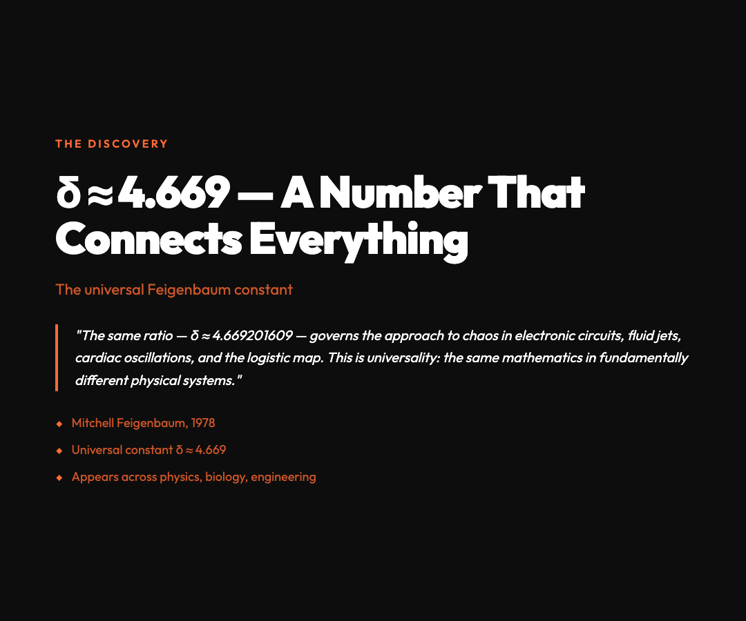
This number is universal. It appears in the logistic map, but also in any system that undergoes period-doubling on the way to chaos — including electronic circuits, fluid jets, and cardiac oscillations. The same ratio governs the approach to chaos in fundamentally different physical systems. That such a specific number could connect biology, physics, and mathematics is one of the stranger facts of twentieth-century science.

Chaos with Windows of Order

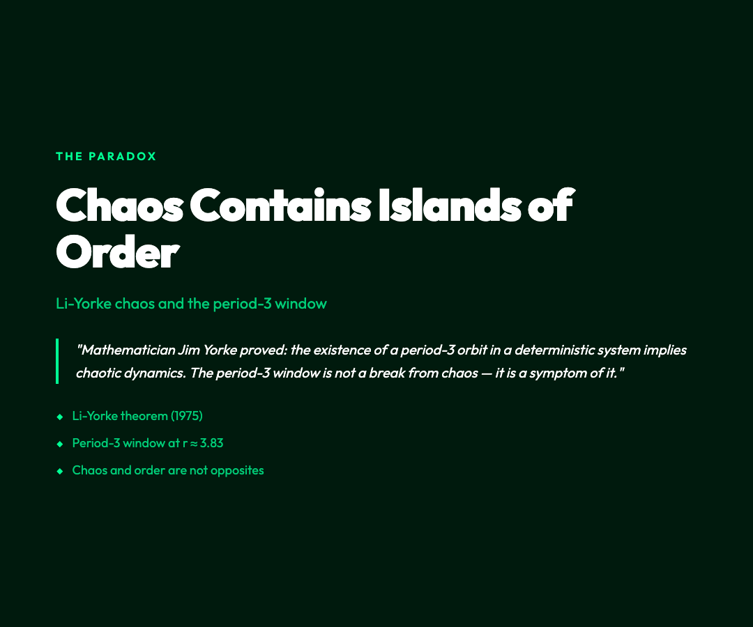
Here is the part that breaks intuition. Within the chaotic regime — the region where the diagram shows a solid smear of unpredictability — there are suddenly bright, narrow vertical windows where order re-emerges. The most famous is the period-3 window near r ≈ 3.83. At exactly this parameter value, the chaos disappears and the system settles into a clean 3-cycle.

This is not a minor quirk. Mathematician Jim Yorke and his student Chung-Wen Li proved something now known as Li-Yorke chaos: the existence of a period-3 orbit in a deterministic system implies chaotic dynamics. The period-3 window is not a break from chaos — it is a symptom of it.

Why the Logistic Map Still Matters

The logistic map is not a toy. It was first proposed to model how animal populations grow and collapse in finite environments — the “1 − x_n” term represents resource limitation. In a given generation, if the population approaches the carrying capacity (x = 1), the growth rate slows and the next generation shrinks.

But the model proved too honest for comfort. Real ecosystems don’t follow smooth equilibrium curves. They overshoot, crash, recover partially, and then oscillate in ways that resist prediction. The logistic map explains why: even this simplest possible model of population dynamics produces chaos at realistic parameter values.

The same mathematics shows up today in epidemiology (modeling how diseases resurge after control measures), in electrical engineering (understanding when a feedback circuit will oscillate versus drift into noise), and in financial modeling (where some practitioners use discrete maps to capture the fat-tailed returns distributions that continuous models systematically miss).

What the Interactive Visualization Shows

The logistic map visualization at ElysiaTools lets you move through this landscape yourself. Three complementary views are available:

The Time Series shows x_n plotted against iteration number n. You can watch a population climb, stabilize, oscillate, and finally dissolve into apparent noise — all by adjusting a single parameter.

The Cobweb Plot draws the characteristic staircase that folds the x-axis onto the parabola x_{n+1} against x_n. When the system is stable, the staircase spirals inward. In a 2-cycle, it traces a rectangle. In chaos, it fills the square without ever settling.

The Bifurcation Diagram is the overview: all possible long-run behaviors simultaneously, across all r values. Zoom in on any region and you will find the same branching structure repeating at finer and finer scales — self-similarity across scales, a hallmark of fractal geometry.

The Core Insight

The logistic map is a machine for understanding the difference between complicated and complex. A complicated system has many parts that interact in knowable ways. A complex system follows simple rules that produce behavior that cannot be long-range predicted — not because we lack information, but because prediction itself is asymptotically impossible past a certain horizon.

That horizon — the onset of chaos at r ≈ 3.56995 — is sharp and deterministic. Cross it and the future becomes genuinely unknowable in a way that a stable system never is. The equation does not change. Only r changes.

But the world it describes transforms completely.

Try it: Logistic Map Visualization — adjust the growth rate r and watch the system move between order and chaos in real time.