Why Square Waves Are Made of Circles (And What That Reveals About Reality)

The square wave looks nothing like a circle. It snaps up, holds flat, snaps down, holds flat — again and again. A circle bends gently in one direction forever. The square wave changes direction instantaneously, four times per cycle. Yet buried inside the square wave is an infinite number of circles, all orbiting at different speeds.

This is not a metaphor. It is Fourier’s theorem, and it is one of the most surprising facts in all of mathematics.

The Warm-Up: Adding Two Circles

Start with the simplest circle. A point traces a sine wave as it goes around. One revolution per second gives you one cycle of sine per second, or 1 Hz.

Now add a second circle, half the size, spinning three times per second. The big circle traces its sine. The small circle traces its own sine, oscillating three times faster and with a smaller amplitude. Add the two together — at each instant, add their vertical positions — and you get something new. Not a pure sine. Not a pure circle. Something in between.

That “in between” shape is your first approximation toward a square wave.

Add a third circle, one-third the size, spinning five times per second. The combined path gets closer to the square shape. Add a fourth at one-fourth the size, spinning seven times per second. Each new circle — each new harmonic — bends the combined path a little more sharply at the corners.

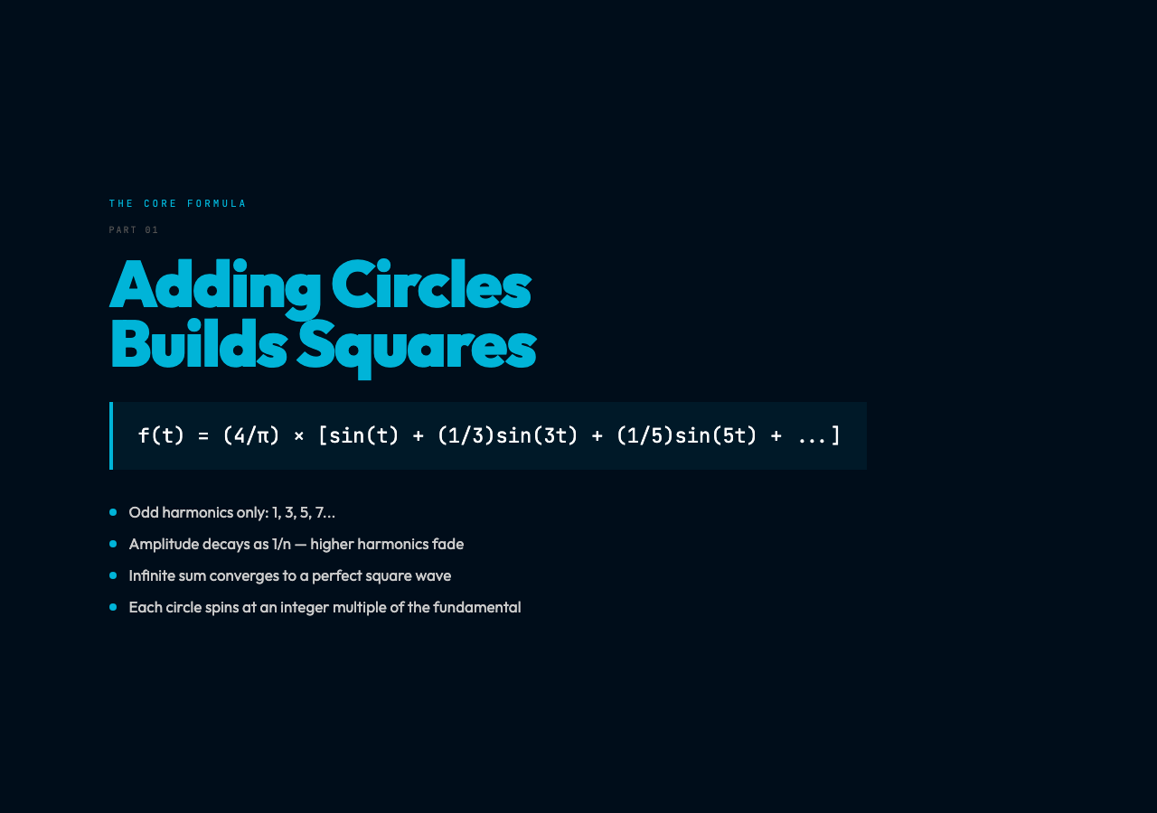
The formula for a square wave captures this exactly:

f(t) = (4/π) × [sin(t) + (1/3)sin(3t) + (1/5)sin(5t) + (1/7)sin(7t) + …]

Each term is a circle spinning at an odd frequency (1, 3, 5, 7…), shrinking in amplitude by the inverse of its frequency (1, 1/3, 1/5, 1/7…). The sum of infinitely many such circles converges to a square wave.

Why This Works: Orthogonal Bases

Fourier’s insight was that the set of sine and cosine functions form an orthogonal basis for a large class of periodic functions — much like (1, 0), (0, 1), and (1, 1) form a basis for two-dimensional space.

Orthogonal means each function has “no overlap” with the others when you measure their inner product over one full period. Just as you can uniquely describe a point in 2D as a combination of x and y coordinates, you can uniquely describe a periodic function as a combination of sine and cosine harmonics. The coefficients tell you how much of each harmonic is present.

For a square wave, only the odd harmonics appear — 1, 3, 5, 7… — and their amplitudes follow the 1/n pattern. For a sawtooth wave, all harmonics appear (both odd and even), with amplitudes of 1/n. Each wave shape has its own fingerprint in the frequency domain.

This is why a spectrogram of a square wave shows a spike at 1 Hz, another at 3 Hz, another at 5 Hz — and nothing in between. The square wave in the time domain becomes a set of discrete vertical lines in the frequency domain.

The Imperfect Truth: Gibbs Phenomenon

Here is where reality intrudes. The mathematical square wave has infinitely many harmonics and perfectly vertical sides. The physical world has neither infinity nor perfect vertical sides.

If you truncate the series at some finite number of harmonics — say, 50 — you get a very close approximation. But look closely at the corners and you will see something unexpected: each corner overshoots. It does not just reach the target and stop. It rings — it goes past, then rings back, then past again, with decreasing oscillations.

This overshoot is Gibbs phenomenon, named after the physicist Josiah Willard Gibbs, who described it in 1899. No matter how many harmonics you add, the overshoot remains at about 9% of the jump height. Adding more harmonics makes the overshoot narrower in time, but never smaller in amplitude. The infinite series converges everywhere except at the discontinuities, where it converges to the midpoint of the jump.

This is not a flaw in the math or a limitation of the visualization. It is a fundamental property of Fourier series: you cannot perfectly represent a discontinuity with a finite sum of continuous functions.

The Deeper Surprise: Discontinuity from Continuity

Square waves are not just mathematical curiosities. They appear everywhere in the real world.

A digital signal in a computer circuit is a square wave — or as close as the hardware can manage. Audio engineers use square waves to test amplifiers: if an amplifier can cleanly reproduce a 1 kHz square wave, it can cleanly reproduce any waveform, because that square wave contains all the frequencies up to very high orders. A crisp, clean square wave tells you the amplifier handles high frequencies well.

Yet every physical square wave is an approximation. The actual voltage does not snap instantly from 0V to 5V. It rises as fast as the circuit allows, which is limited by parasitic capacitance and inductance. The sharper the intended edge, the more high-frequency harmonics the signal contains. A 1-nanosecond edge contains frequency components up to roughly 350 MHz — far beyond the fundamental.

This is why microwave engineers think in the frequency domain. A “discontinuity” in time — an edge — is not a mysterious event. It is the sum of many circles, many sinusoids, each one continuous and smooth. Reality, at the level of Maxwell’s equations, is always continuous.

From Waves to Understanding

The Fourier perspective transforms how you see periodic phenomena. A heartbeat is not just a pressure waveform in time — it is also a spectrum of frequencies, each corresponding to a different harmonic, each telling you something about the physiology. A musical instrument playing an A note at 440 Hz is not producing a pure 440 Hz sine wave. It is producing 440 Hz plus 880 Hz, plus 1320 Hz, plus higher harmonics at different amplitudes and phases. The unique mix of harmonics is what distinguishes a violin playing A from a flute playing the same note.

Fourier’s theorem says these two descriptions — the time-domain waveform and the frequency-domain spectrum — contain exactly the same information. You can convert between them without loss. The waveform tells you what the signal looks like moment to moment. The spectrum tells you what frequencies are present and in what proportions.

This dual description is not just a mathematical trick. It is how engineers design audio systems, how astronomers analyze starlight, how doctors interpret EEGs and EKGs, and how compression algorithms like MP3 decide what parts of a music file you can safely discard without hearing the difference.

The square wave, made of circles, is the simplest demonstration of this duality. Start with one circle. Add a second at three times the frequency. Watch the sum approach a square. Gibbs phenomenon appears at the corners — the price of representing a discontinuity with continuous functions. The overshoot never fully goes away. And that limitation, that permanent gap between the mathematical ideal and the physical approximation, is itself a deep truth about the nature of functions, continuity, and the limits of representation.

Reality is continuous. Our signals are not. The bridge between them is an infinite sum of circles.