Roll a fair die 10,000 times and record every outcome. The histogram is flat — each face appears roughly 1,667 times, no more, no less. That is exactly what you would expect from a uniform distribution. Now do something different: roll the die 30 times, write down the average, repeat until you have 333 averages, and plot those on a histogram. What shape do you see?
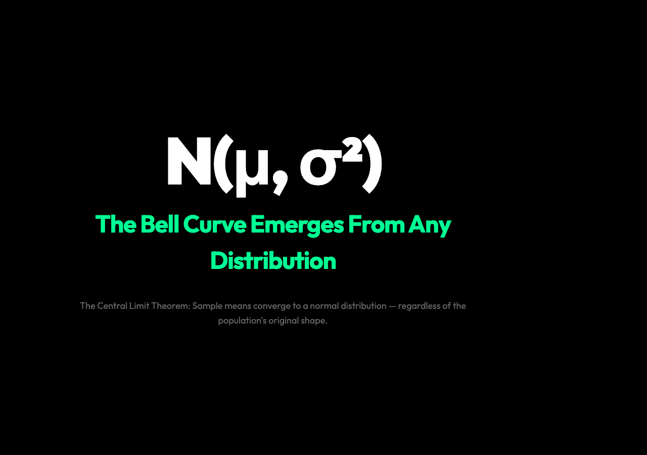
Not flat. A bell curve. No matter how many times you repeat this — from a die, a loaded coin, a radioactive decay, a stock price — the distribution of sample means always converges to the same shape. That is the central limit theorem, and it works even when the underlying process looks nothing like a bell.
The Puzzle: When Averaging Creates Order
The central limit theorem describes what happens when you draw samples from any distribution — yes, even a flat uniform, an exponential decay, or a weird two-humped bimodal spike — and look at the distribution of the means of those samples. The theorem states that the histogram of sample means converges to a normal (Gaussian, bell-curve) distribution, regardless of the population’s original shape. You do not need the original data to be normal. You do not need to know the population’s shape at all.
This is surprising because it runs against how we normally think about distributions. If you sample from a uniform distribution, you expect uniform results. If you sample from an exponential distribution, you expect exponential results. But the mean of samples is not the same thing as a sample. Averaging is a different operation, and it produces a different output — one that, for deep mathematical reasons, always settles into the same shape.
The Standard Error: How the Spread Shrinks
There is a precise formula for how concentrated those sample means are. The standard deviation of the sample means — called the standard error — is equal to the population’s standard deviation divided by the square root of the sample size:
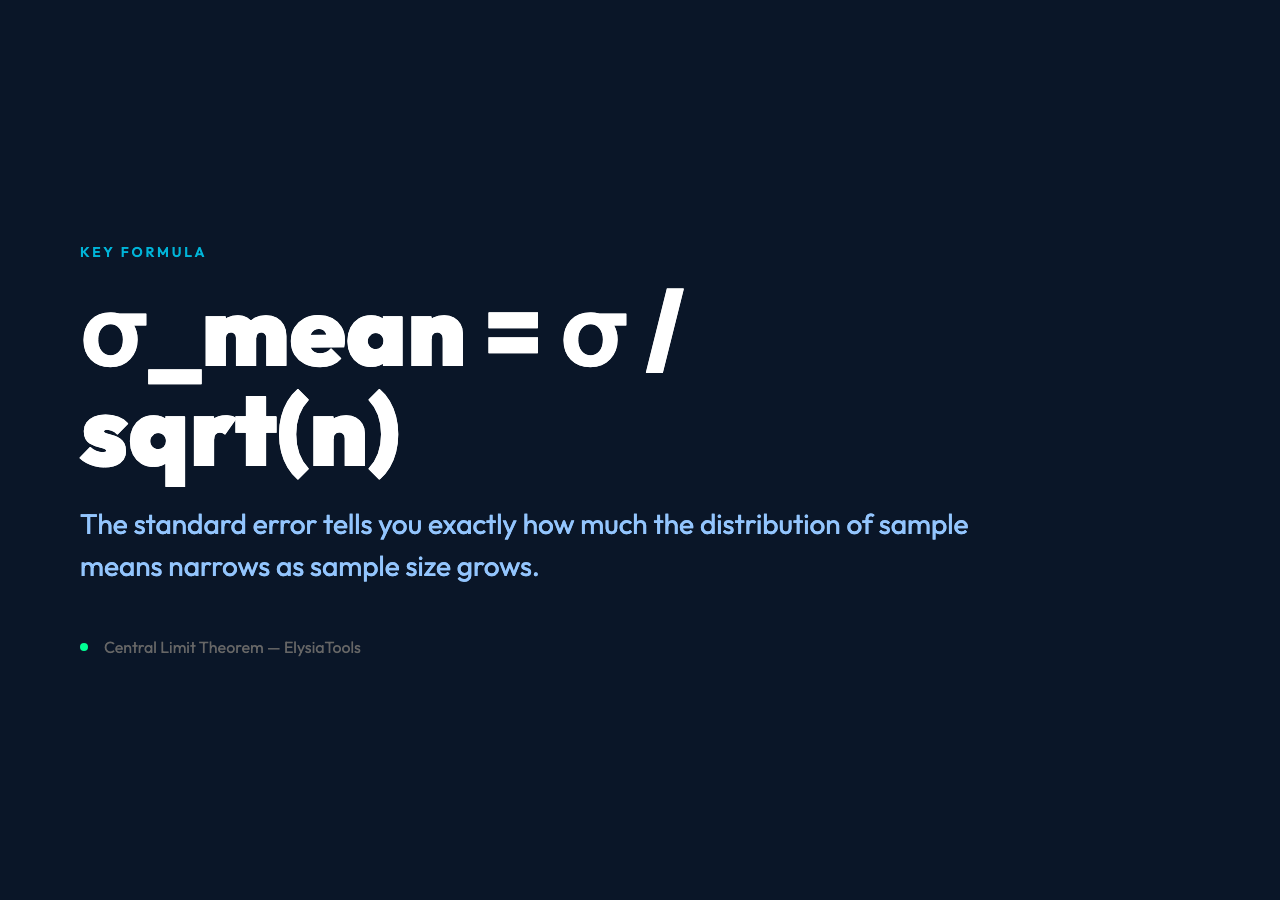
σₘₑₐₙ = σ / √n
If the population has σ = 1 and you sample n = 30 at a time, the standard error is 1/√30 ≈ 0.18. If you increase n to 100, the standard error drops to 0.10. The histogram of sample means gets narrower and taller as n grows, but its shape is always a bell curve.
Six Distributions, One Destination
The ElysiaTools Central Limit Theorem visualizer lets you test this yourself. You can choose from six population distributions:
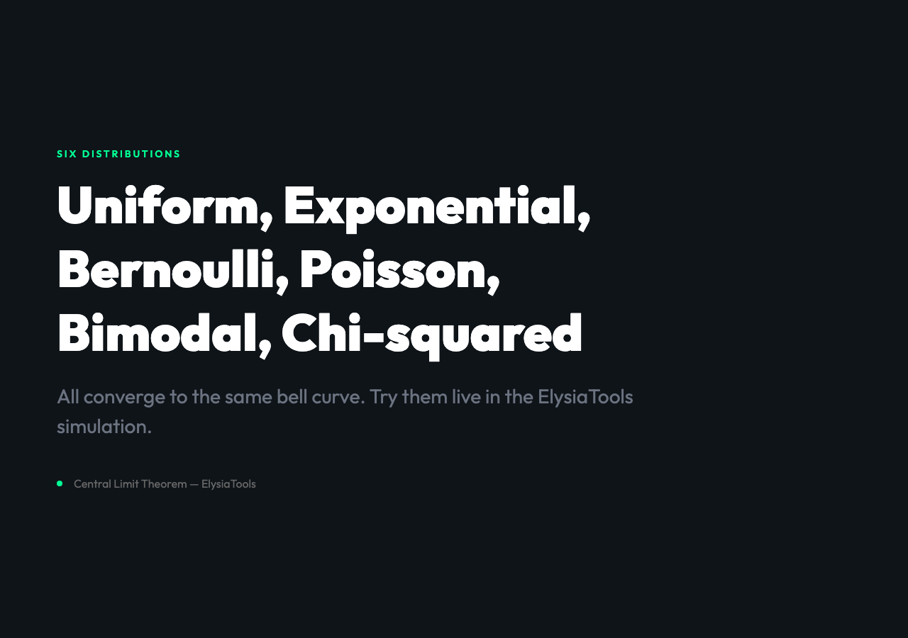
- Uniform: flat from 0 to 1
- Exponential: decaying — most values cluster near zero
- Bernoulli: binary, 0 or 1
- Poisson: discrete counts clustered around a mean
- Bimodal: two separate peaks at −2 and +2
- Chi-squared: right-skewed with a long tail
Set the sample size to 30 and the animation speed to fast. Watch as the histogram in the bottom panel — the distribution of sample means — forms a near-perfect bell curve, even though the population panel above it shows something completely different. The convergence is fast. You will see a recognizable bell shape after fewer than 200 samples in most cases, even from the bimodal or chi-squared distributions which look nothing like a bell curve at the population level.
Why This Happens: The Mathematics of Aggregation
The reason is not magic — it is the mathematics of adding independent random variables together. When you take n independent draws from any distribution and average them, you are performing a sum (or a sum scaled by 1/n). The sum of independent random variables tends toward a normal distribution through a mechanism related to the law of large numbers and the central limit theorem proper (Lindeberg-Levy form).

The intuition is this: any irregular distribution, when you sample from it enough times and add those values together, produces a sum that is the superposition of many small, independent sources of variation. By the law of large numbers, those many small contributions wash out the idiosyncratic structure of the original distribution and leave only the shared, universal pattern. The Gaussian is the fixed point of the convolution operation — apply it often enough to any starting distribution, and you get the same thing back.
Why It Matters: From Polling to Quality Control
The central limit theorem is the engine behind almost every practical application of statistics. When pollsters survey 1,000 people to estimate how an entire country will vote, they are relying on the CLT: the sample mean will be approximately normally distributed around the true population proportion, with a standard error that shrinks as √n grows. This is why bigger samples give more precise estimates — not because they capture more of the population directly, but because the mean of the sample benefits from the CLT’s convergence. A poll of 1,000 people can estimate the views of 330 million.
In manufacturing, quality control charts use the CLT to set control limits. A machine that produces parts with a mean of 100g and standard deviation of 2g will produce sample means that follow a normal distribution. Any single part might be 95g or 107g — within natural spread. But if the average of 5 consecutive parts drifts above 103g, that signal is statistically meaningful in a way that a single outlier reading is not.
In finance, portfolio returns are analyzed as sums of correlated asset returns. The CLT underlies Value at Risk models and the justification for treating diversified portfolios as approximately normal, even when individual asset returns are fat-tailed and far from normal themselves.
Here is the question worth sitting with: if the CLT works this well on distributions that look nothing like a bell curve — a uniform flat, a decaying exponential, a double-humped bimodal spike — then what other universal patterns are hiding inside aggregations we have not looked at closely enough? The theorem guarantees the shape of the answer. The more interesting question is which other phenomena, currently buried in messy data, would reveal their own hidden symmetries under the same operation.