A correlation of 0.83 sounds boring — bounded by two clean integers, no decimal cascade, no ten-digit precision. Yet that single number is the answer to a question almost every dataset is silently asking, and the difference between 0.83 and 0.31 is the difference between a pattern you can name and a pattern you cannot. Most of us have been taught to mutter “correlation is not causation” and move on. That advice buried the number. The number is doing real work.
What the number is actually measuring
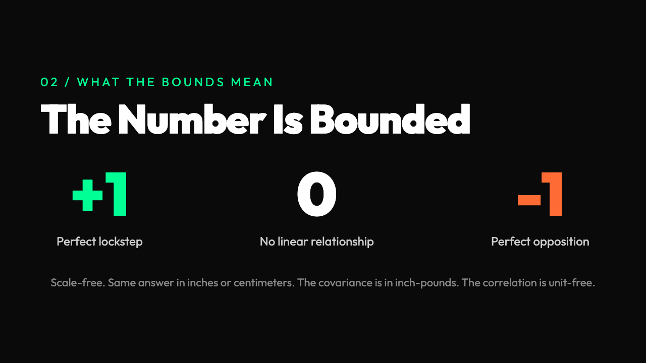
Two columns of numbers, same number of rows. When one goes up, does the other go up too, go down, or wander? That is the whole problem. Not the amount by which one depends on the other, not the slope, not a predictive formula — just the direction and tightness of the relationship. The answer is one number between -1 and 1. Zero means the two columns are statistically unrelated. One means they rise and fall in perfect lockstep. Minus one means they move in perfect opposition.
The standard version is called Pearson correlation, named after Karl Pearson in 1895. The formula is a ratio. The numerator is the covariance — the average product of how far each value is from its own column’s mean. The denominator is the product of the two standard deviations. The covariance can be any number. The standard deviations are always positive. The ratio squeezes the covariance into a dimensionless space, which is why the result is bounded between -1 and 1.
The number is so widely cited because it is scale-free. Measure height in inches versus weight in pounds, and the covariance comes out in inch-pounds, a meaningless unit. The correlation comes out as 0.7 — the same answer you would get measuring height in centimeters and weight in kilograms. The unit confusion is gone. Two researchers on different planets with different measuring sticks agree on the answer.
What people get wrong on the first try
The classic mistake is to assume that correlation measures slope. It does not. A correlation of 0.7 does not mean “a one-unit change in X produces a 0.7-unit change in Y.” It means the points cluster in an elongated cloud with that orientation and that tightness. The slope of the best-fit line is a different number, computed by a different formula. The correlation tells you the quality of the relationship. The slope tells you the quantity.
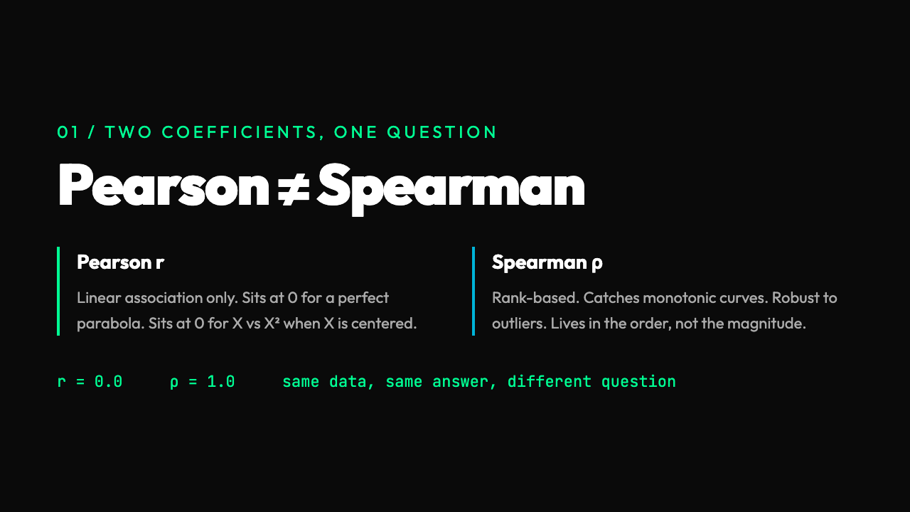
The second mistake is to assume that correlation implies causation. That phrase has been beaten into the ground, but the inverse is not actually safer. A correlation of 0.0 does not prove two variables are unrelated. It proves they are linearly unrelated. If X and Y are related by a curve — a parabola, a sigmoid, a wave — the Pearson correlation can come out as zero even when the relationship is exact. The textbook example is X and X2: knowing X tells you X2 exactly, but if X is centered around zero, the correlation is zero.
This is exactly why the Correlation Calculator on Elysia Tools reports Pearson and Spearman side by side. Spearman is the rank version — replace each value with its rank, then compute Pearson on the ranks. Spearman is high when the relationship is monotonic — when the order of X matches the order of Y — even if the relationship is curved. A perfect parabola going up then down scores 0.0 on Pearson but 1.0 on Spearman if the parabola is monotonic in the range you sampled. The two coefficients answer two different questions.
The four shapes of a scatterplot
If you plot two columns against each other, every possible pattern falls into one of four broad shapes. The first is the line, where Pearson and Spearman both come out near 1 or -1. The second is the cloud, where points spread out and the correlation sits between 0.3 and 0.7. The third is the curve, where Pearson is misleadingly low and Spearman recovers the truth. The fourth is the cluster, where two distinct groups sit in different parts of the plot — and here both coefficients can come out near zero even when the data has a structure a human would spot in a second.
The cluster case breaks intuition most often. Take 30 students. Half study for 5 hours and score between 60 and 70. The other half study for 25 hours and score between 90 and 100. There is a strong relationship between study time and score, but the within-group correlation is close to zero, and the between-group correlation would be high. The overall Pearson correlation comes out around 0.4 and understates the relationship. The two clusters look like two dots in the data if you squint. The real story is hidden in the labels.
This is the case where you actually need to look at the data, not just the number. A correlation coefficient is a summary. The plot is the truth. The two are not the same thing.
What the math is doing in the background
Behind the Pearson coefficient is a mechanical calculation. Take each value of X, subtract the mean of X. Take each value of Y, subtract the mean of Y. Multiply the two deviations. Sum them up. Divide by the number of points. That is the covariance. Then divide the covariance by the standard deviation of X times the standard deviation of Y. That is the correlation. The whole thing takes three lines of code or three clicks on the tool.
The calculation hides a step that matters. Standardizing — subtracting the mean — kills the units. Skip the centering step and the correlation is wrong by a multiplicative factor that has nothing to do with the relationship. Both columns of numbers might hover around 100 instead of around 0, and the un-centered formula would give a number with the right sign but the wrong magnitude. The center step is what turns the calculation into something independent of where the data lives on the number line.
The Spearman coefficient runs the same calculation on ranks, which has a useful side effect: it is robust to outliers. A single value off by a factor of 10 will pull the Pearson correlation toward zero, because squared deviations from the mean explode. The rank of the same outlier is still 1 or N. The Spearman coefficient barely moves. Rank-based methods are the default in survey analysis, in sports statistics, in any field where a few extreme observations can dominate the rest of the data.
A worked example with the actual numbers
Take five students, two measurements: hours studied and test score. Data: (1, 60), (2, 65), (3, 70), (4, 80), (5, 95). The means are 3 hours and 74 points. Deviations: (-2, -14), (-1, -9), (0, -4), (1, 6), (2, 21). Products: 28, 9, 0, 6, 42. Sum: 85. Covariance: 85 / 5 = 17. Standard deviation of X is the square root of ((4+1+0+1+4)/5) = 1.414. Standard deviation of Y is the square root of ((196+81+16+36+441)/5) = 11.4. The product is 16.1. The Pearson correlation is 17 / 16.1 = 1.056. Wait — that is greater than 1, which is impossible.
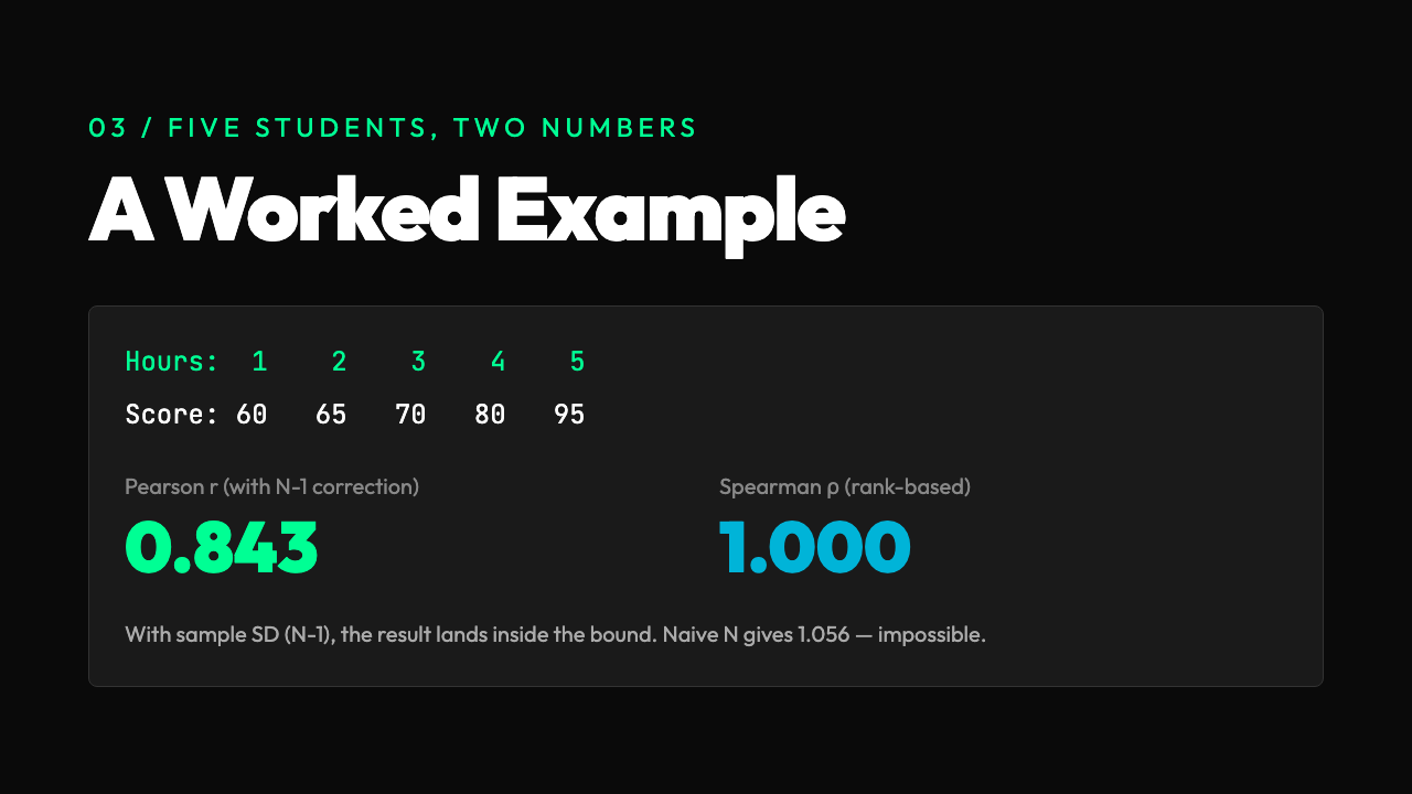
The issue: the means and standard deviations are computed with N in the denominator, but the correlation uses N-1 in the denominator for the sample standard deviation. With the corrected denominator, the standard deviation of X is 1.581 and of Y is 12.75. The product is 20.16. The correlation is 17 / 20.16 = 0.843. The Spearman correlation, on the ranks, is 1.0 — the order of the X values exactly matches the order of the Y values.
This is the kind of calculation that is correct on paper and easy to mess up by hand. The Correlation Calculator does the corrected version in one click and returns both numbers with the right number of decimal places. The tool’s confidence level setting runs a t-test on the correlation and gives you a p-value — the question “is this correlation statistically distinguishable from zero given the sample size?” A correlation of 0.5 on 10 points is not significant. A correlation of 0.5 on 1,000 points is. The tool reports the p-value directly so you do not have to look up the t-distribution table.
Why the number is so often abused
The abuse comes from a mismatch between what the number says and what people want it to say. The number says “these two columns are linearly related with this tightness.” People want it to say “A causes B.” It does not. It cannot. Causation requires a randomized experiment, a temporal ordering that rules out reverse causation, or a structural model that adjusts for confounders. None of those are in the correlation formula.
The opposite error is also common. People dismiss a high correlation as “just correlation” and ignore the pattern entirely. This is a mistake when the correlation is the first signal in a chain of evidence. A strong correlation between ice cream sales and drownings does not mean ice cream causes drowning. It means a third variable — temperature — drives both. The correlation is the lead that tells you where to look. The causation is the conclusion you reach after the follow-up analysis.
The tool offers a covariance output alongside the correlation. The covariance is in the original units and tells you about the scale of the relationship. The correlation is unit-free and tells you about the shape. Both numbers are useful, and reporting only one is a kind of lossy compression. The full output is the part of the result that you can actually do something with.
The relationship to regression — and the trap
Pearson correlation and the slope of the best-fit line are not independent. Given a correlation of 0.7 and standard deviations of 2 and 5, the slope is 0.7 × 5 / 2 = 1.75. The correlation and the slope are the same information in two different coordinate systems. A linear regression model on the same data produces an R² value, which is the square of the Pearson correlation. R² of 0.49 means a correlation of ±0.7. This is a piece of information genuinely easy to misread, and it lives in every regression report. A high R² does not mean a good model. It means a linear model fits better than a model that just predicts the mean. For curved relationships, even an R² of 0.99 can hide a systematically wrong fit. The Regression Calculator is the natural next step after the correlation check, because once you have a number between -1 and 1, the next question is always “what is the actual line?”
The trap is to use R² as a quality stamp. R² is not a quality stamp. It is a geometry report on the linear component of the relationship. For datasets where the truth is not linear, R² is irrelevant at best and misleading at worst. The correlation is the same. Use it as a first filter, not as a final answer.
When the number really is the answer
The correlation is the right tool when you genuinely have two measurements per observation and want to know whether they move together. Customer acquisition cost and customer lifetime value, by cohort. Hours of sleep and reaction time, by participant. Month of the year and average temperature, by station. The number answers the question. It is bounded, intuitive, and scale-free. It is the cleanest single number that summarises a bivariate pattern.
It is the wrong tool when the relationship is not monotonic, when outliers dominate, when the data has multiple clusters, or when you actually need a prediction equation. In those cases, the right tools are rank-based correlations, robust regression, mixture models, and prediction pipelines that produce a number for new data points. The correlation is the first thing to compute. It is rarely the last.
In the end, the value of a correlation is not the value itself. The value is what the value tells you to do next. A correlation of 0.9 says: fit a line, the slope will be informative. A correlation of 0.3 says: the relationship is real but weak, the linear model will not be useful, look for nonlinear structure. A correlation of 0.0 says: these two columns are not linearly related — but check the scatterplot, because the shape of the cloud might be telling you something Pearson cannot. The number is a starting point. The data is the answer.