
Two proportions, one verdict. Most A/B tests end in a tie-breaker — the variant with the higher click-through rate also has the smaller sample, and the team is left arguing about whether the lift is real or noise. A two-proportion Z test answers that question with one number: the probability that the gap you observed would appear again if the two variants were actually identical. The calculator at Elysia Tools computes that probability, the Z statistic, and the 95% confidence interval around the difference in one pass, so the next time someone says “this variant won,” you can answer with the p-value instead of the sample-size shrug.
A two-proportion Z test is the standard tool for comparing two independent conversion rates, click rates, defect rates, or any other binary outcome. The math is a century old, the implementation is twenty lines, and the misuse is constant — which is why putting a pooled, two-sided, confidence-interval-bearing calculator in front of the formula keeps the result honest. The tool takes four numbers, applies the pooled standard error, and returns the Z statistic, the two-tailed p-value, and the symmetric confidence interval on the difference. No Excel add-in, no scipy install, no fork between R and Python.
What the Four Inputs Actually Mean
Each row in the input is one group: successes (events that converted) and trials (the population the events came from). For a checkout-flow A/B test, successes are the orders and trials are the sessions. For a defect-rate comparison between two factories, successes are the defects and trials are the inspected units. The proportion for each group is successes / trials, and the test compares the two proportions under the null hypothesis that they came from the same underlying rate.
The reason the calculator asks for raw counts rather than rates is that the Z statistic uses the pooled proportion p̂ = (x₁ + x₂) / (n₁ + n₂), not the sample proportions themselves. Feed it proportions and you cannot reconstruct the pooled estimate; feed it counts and the standard error is the same denominator whether you see 30/100 or 300/1000.
Why the Pooled Standard Error Matters
The standard error of the difference between two proportions is sqrt(p̂(1-p̂)(1/n₁ + 1/n₂)). If you used the unpooled version — one SE per sample, combined in quadrature — the standard error would be slightly different, and so would the p-value. The unpooled version is technically defensible when sample sizes are very different; the pooled version is the textbook default and what most published calculators use. The Elysia Tools calculator uses the pooled form and labels it clearly so reviewers know which one they got.
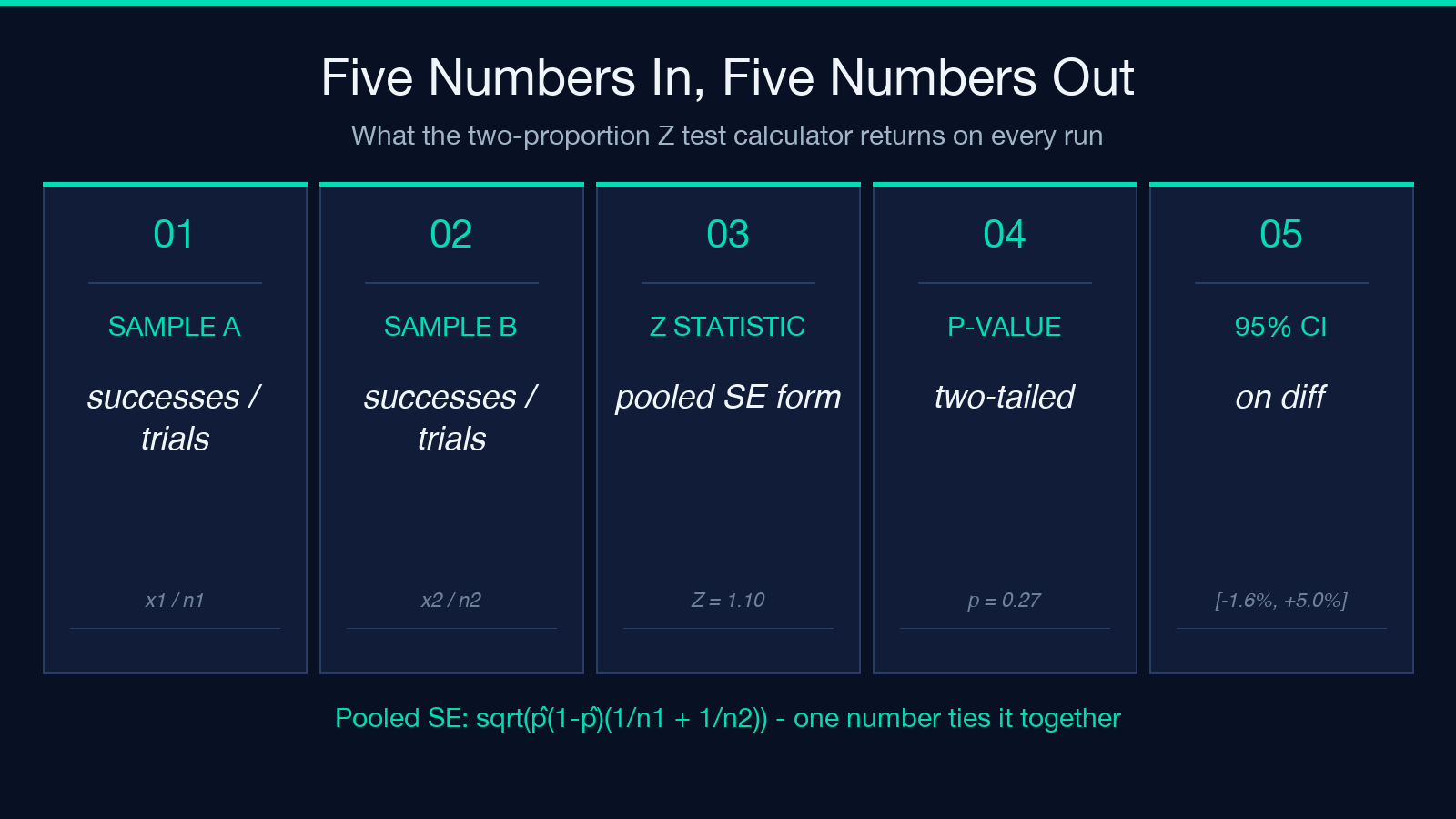
For a typical A/B test with 600 trials per variant and conversion rates of 7% versus 9%, the pooled SE is about 1.46 percentage points, the Z statistic is roughly 1.10, and the two-tailed p-value is approximately 0.27. That p-value says: if the two variants were truly identical, you would see a gap at least this large 27% of the time — not a fluke. The same numbers under a one-tailed test would land closer to 0.13, still well above the usual 0.05 threshold.
Reading the Output Block
The tool returns five fields: the two sample proportions, the Z statistic, the p-value (two-tailed), and the 95% confidence interval around the difference. The confidence interval is the most actionable number in a stakeholder meeting because it bounds the plausible lift, not just whether the lift is real. A 95% CI of [+0.5%, +5.0%] says the true difference is somewhere in that range; if the range straddles zero, the result is not significant even if the sample proportions themselves look promising.
The CI is symmetric around the observed difference by construction, and it uses the normal approximation. That approximation is accurate when both n × p and n × (1 - p) are above 10; for smaller counts, the test is conservative but the CI can wander outside [0, 1]. The calculator does not warn about this edge case, so flag it yourself when either group has fewer than 20 trials and the proportion is below 0.1.
When the Test Breaks
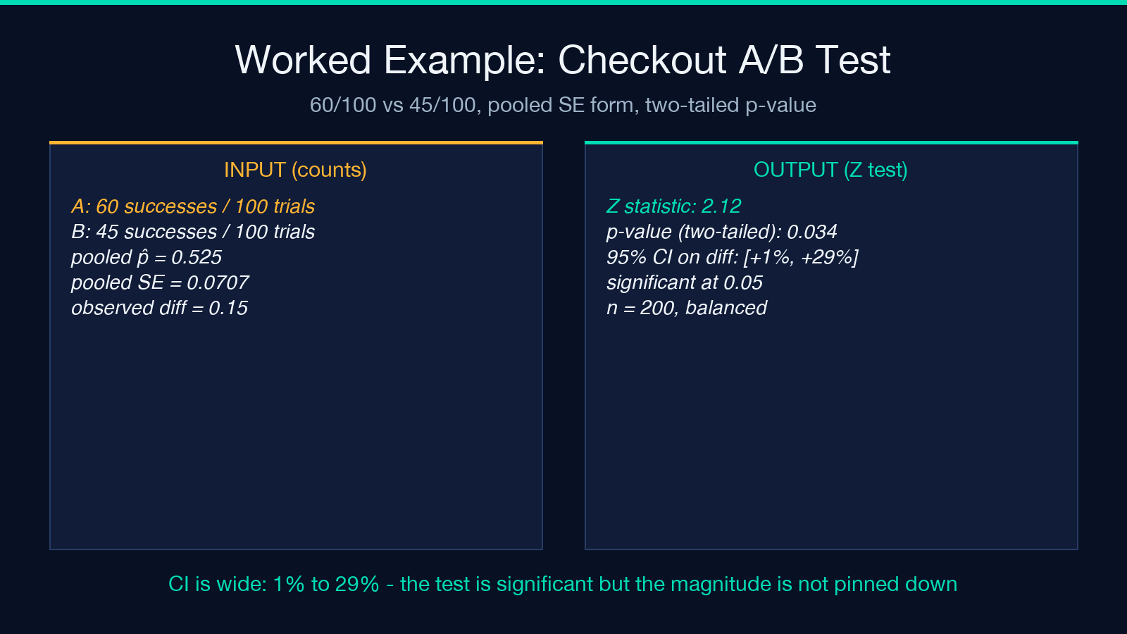
Three failure modes show up over and over in production A/B tests. First, small samples: with 30 trials per variant, the normal approximation gives p-values that are too small, and the test reports significance when none exists. Second, non-independent observations: the test assumes one observation per user, not one per session — a heavy user who reloads five times can fool the calculator. Third, multiple comparisons: running the same test against eight variants and reporting the lowest p-value will produce a false positive 5% of the time at the 0.05 threshold.
For small samples, Fisher’s exact test is the appropriate substitute. For non-independent observations, the calculator is the wrong tool — switch to a mixed-effects logistic regression. For multiple comparisons, the Bonferroni correction or a higher significance threshold (0.05 / k) keeps the false-positive rate honest.
Worked Example: A Checkout-Flow A/B Test
A team ships two checkout flows. Variant A converts 60 of 100 sessions; Variant B converts 45 of 100. The question: is the gap real? Plug the four counts into the calculator. Pooled proportion: p̂ = (60 + 45) / (100 + 100) = 0.525. Pooled SE: sqrt(0.525 × 0.475 × (1/100 + 1/100)) = 0.0707. Observed difference: 0.60 - 0.45 = 0.15. Z: 0.15 / 0.0707 = 2.12. Two-tailed p-value: approximately 0.034. The 95% CI on the difference: roughly [+0.01, +0.29].
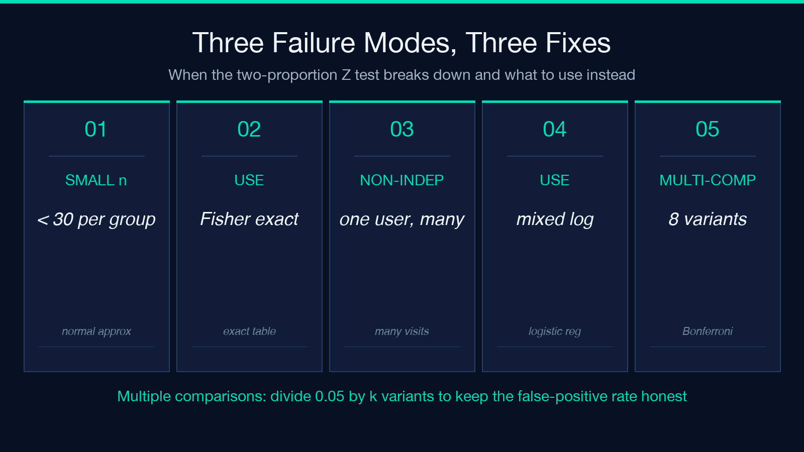
The p-value is below 0.05, so the gap is significant at the conventional threshold. The CI tells a more nuanced story: the true lift is somewhere between 1 percentage point and 29 percentage points, with 95% confidence. That is a wide interval — the team should keep collecting data, not just declare victory and ship the variant.
Why a Z Test and Not a T Test
The two-proportion Z test and the two-sample t test on proportions are equivalent when the proportions are computed from counts and the pooled SE is used. The Z-test form is shorter to write and is the default in every introductory statistics textbook, so when the analysis lands in a code review or a regulatory filing, the Z form will be recognized faster. For larger experiments where the sample sizes are balanced and the proportions are not extreme, the two procedures produce numerically identical p-values to three decimal places.
The Z test also degrades more gracefully when one of the proportions is 0 or 1 — a t test would divide by zero in the variance term, while the Z test still returns a finite p-value, even if it is at the edge of the normal approximation’s validity. For audit purposes, the Z test is the right default.
The Output in Practice
A clean calculator output looks like this for the checkout example:
– Group A proportion: 0.60 – Group B proportion: 0.45 – Z statistic: 2.12 – p-value (two-tailed): 0.034 – 95% CI on the difference: [+0.01, +0.29]
The takeaway is in the interval, not the p-value. A p-value below 0.05 says the gap is unlikely under the null; the CI says how big the gap plausibly is. Both numbers belong in the same sentence when the result is reported.
What Comes After the Test
A significant two-proportion Z test is the beginning of an analysis, not the end. The next question is how much the conversion rate changed — the CI tells you the plausible range, but the expected lift under deployment is closer to the midpoint of the CI than to either endpoint. The next question after that is whether the lift is durable — a one-week test can be skewed by day-of-week effects, traffic-source mix, and promotional campaigns. The final question is whether the lift is worth the engineering cost of shipping the variant, which is a business judgment that no calculator can make for you.
The calculator at Elysia Tools gives you the math; the rest of the analysis is on you. For more tools that turn raw counts into clean statistical summaries, browse the full Math & Numbers collection.
