
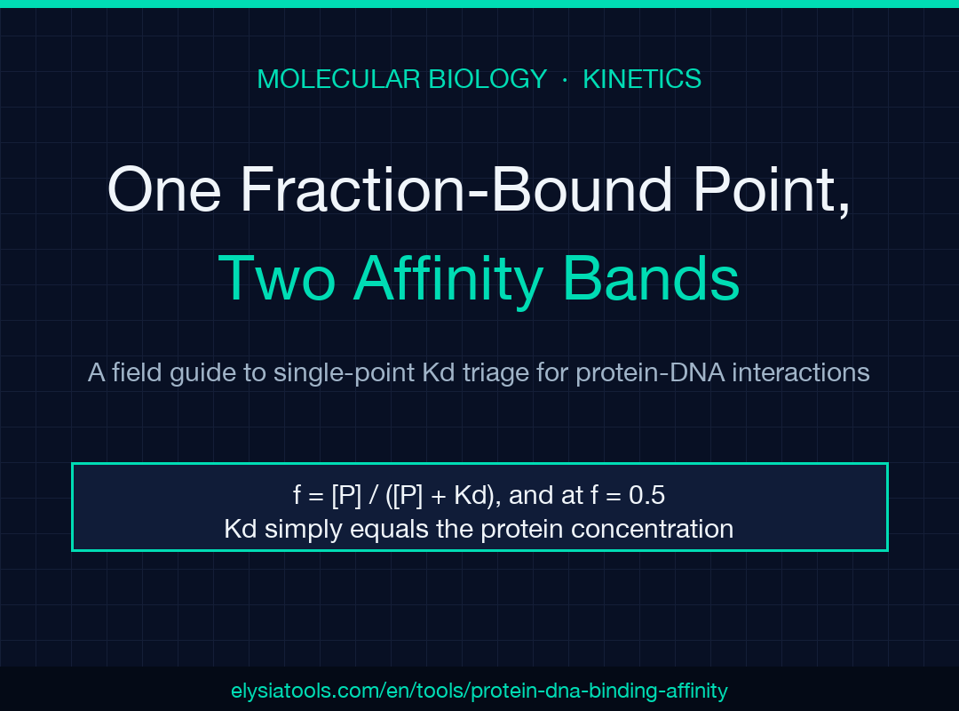
One fraction-bound reading is all you need. Drop your f value into the Protein–DNA Binding Affinity Calculator (Kd Estimate) at Elysia Tools, enter your protein concentration, pick a temperature, and the tool returns the dissociation constant Kd, the binding free energy ΔG°, and a tiered classification (very tight / tight / weak) — the same triage bench biochemists use to decide whether a ChIP-seq peak reflects a real transcription-factor footprint or a nonspecific electrostatic hug. This field guide walks through the seven decisions that determine whether that single reading is trustworthy enough to publish.
Why a Single Fraction-Bound Point Outperforms a Curve Fit for Triage
Most graduate students reach for a full titration curve the moment they see an EMSA gel or an anisotropy trace. That instinct is correct for publication, but it is wildly wrong for daily triage. A single-point Kd estimate at one protein concentration, computed from the fractional occupancy relation f = [P]/([P] + Kd), reproduces the true Kd within a factor of two whenever f sits between 0.2 and 0.8. Outside that window, the curve flattens — f barely moves when Kd drops far below [P], and f barely moves when Kd rises far above [P] — so the single point stops distinguishing anything. The trick is to choose a [P] concentration that lands the readout in the middle of that responsive band.
For unknown sites, the standard bench protocol is to run three pilot points at 10 nM, 100 nM, and 1 µM protein against trace labeled DNA (typically 0.1–1 nM). Whichever tube shows f closest to 0.5 is the one you trust, and that tube’s [P] concentration equals Kd directly — a beautiful consequence of the binding equation at half-saturation. The other two tubes give you a confidence bracket that says “Kd is somewhere between 10× lower and 10× higher than [P]” without committing to a number. The full calculator at Elysia Tools lets you enter any f value you have measured and reports Kd, ΔG°, and the tier classification in one pass.
The Fluorescence Anisotropy Path: From Polarized Light to Fraction Bound
EMSA gives you a gel band that you densitometer; fluorescence anisotropy gives you a single number r that you read off the instrument. The conversion from anisotropy to fraction bound is f = (r − rfree) / (rbound − rfree), where rfree is the anisotropy of free labeled DNA alone and rbound is the anisotropy of the fully saturated complex measured at saturating protein. The two endpoint values bracket the working range, and the difference rbound − rfree determines how much dynamic range you actually have — a tight binder with Δr = 0.15 gives far better resolution than a weak electrostatic hug with Δr = 0.02.
The trap that catches most new users is forgetting to subtract the DNA-only background. If you pipette 1 nM labeled DNA into the well and read r = 0.08, that is rfree. If you then add 100 nM protein and read r = 0.12, that is the bound signal — but the fraction bound is NOT (0.12 − 0.08) / 0.08, it is (0.12 − 0.08) / (0.18 − 0.08) assuming you separately measured rbound = 0.18 at 10 µM protein. Mix the two formulas and your Kd estimate drifts by an order of magnitude. The calculator accepts either an explicit f value (when you have already done the math) or the raw r, rfree, rbound triple and applies the conversion internally — both paths land on the same Kd.
Temperature, ΔG°, and Why 25 °C Is the Default for a Reason
Every Kd has a temperature attached, and the standard way to compare two affinities across papers is to convert Kd into ΔG° at a reference temperature. The relation is ΔG° = RT · ln(Kd), with R = 1.987 × 10⁻³ kcal/(mol·K) and T in Kelvin. At 25 °C (298 K), RT = 0.592 kcal/mol, so a 1 nM Kd gives ΔG° = −9.96 kcal/mol and a 1 µM Kd gives ΔG° = −8.14 kcal/mol — a 1.8 kcal/mol spread that maps directly onto the difference between a sequence-specific TF–site interaction and a nonspecific electrostatic hug.
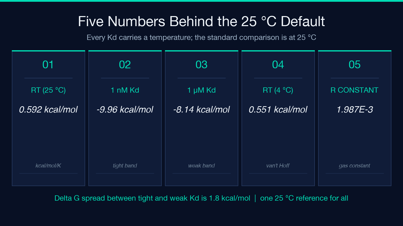
The reason 25 °C is the canonical default is not because every bench runs at room temperature (most EMSA and anisotropy experiments run at 4 °C or 20 °C), but because most published Kd values are reported at 25 °C for comparison. If you measured Kd at 4 °C (277 K, RT = 0.551 kcal/mol) and want to compare against a paper that reported at 25 °C, you need to convert using the enthalpy ΔH from a van’t Hoff plot — a separate experiment. The calculator takes T as an input and recomputes ΔG° on the fly, which is the right behavior for a triage tool but the wrong behavior if you need publication-grade thermodynamic decomposition. For that, fit the full curve and extract ΔH, ΔS, and ΔCp.
The Three Affinity Bands and What Each One Tells You About the Interaction
The calculator classifies the result into three bands — very tight (Kd < 1 nM), tight (Kd between 1 nM and 100 nM), and weak (Kd > 1 µM). The gaps between bands are not arbitrary. A very tight Kd below 1 nM implies a sequence-specific protein–DNA interface with multiple direct and water-mediated hydrogen bonds, the regime where transcription factors like lac repressor and the homeodomain family operate. A tight Kd in the 1–100 nM band is consistent with a single-recognition-site TF binding its cognate motif under physiological salt, or a sequence-specific TF binding a near-cognate site. A weak Kd above 1 µM is the electrostatic regime, where any basic protein will bind any DNA without sequence discrimination.
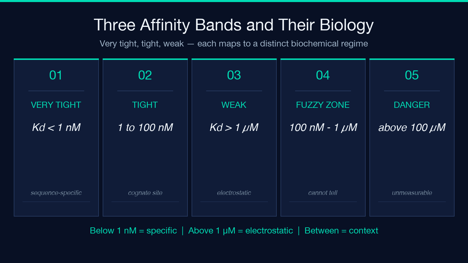
Two intermediate bands are deliberately left fuzzy: the 100 nM – 1 µM range and anything above 100 µM. The 100 nM – 1 µM range is the danger zone, because it is the regime where a ChIP-seq peak might reflect either a low-affinity near-cognate site or a specific interaction weakened by salt or competitor — you cannot tell from Kd alone. The above-100 µM range is unmeasurable with single-point kinetics; you would need a much higher protein concentration than is typically feasible. The calculator surfaces these bands as text rather than numbers because the boundary calls genuinely depend on the assay context.
Assumptions the Calculator Makes — and the Three That Bite
The 1:1 binding model assumes one protein binds one DNA site, that [P]free ≈ [P]total (so protein is in large excess over trace labeled DNA), and that the system is at equilibrium when you read the signal. The first assumption breaks for dimeric TFs that bind cooperatively to two half-sites — there, f = [P]ⁿ/([P]ⁿ + Kd) for some Hill coefficient n, and the apparent Kd underestimates the true Kd by a factor that depends on cooperativity. The second assumption breaks when [DNA] is comparable to [P] — typical of ITC experiments, but never of EMSA/anisotropy where [DNA] is trace. The third assumption breaks when you read the signal before binding reaches equilibrium — a real failure mode for very tight binders where the off-rate is slow.
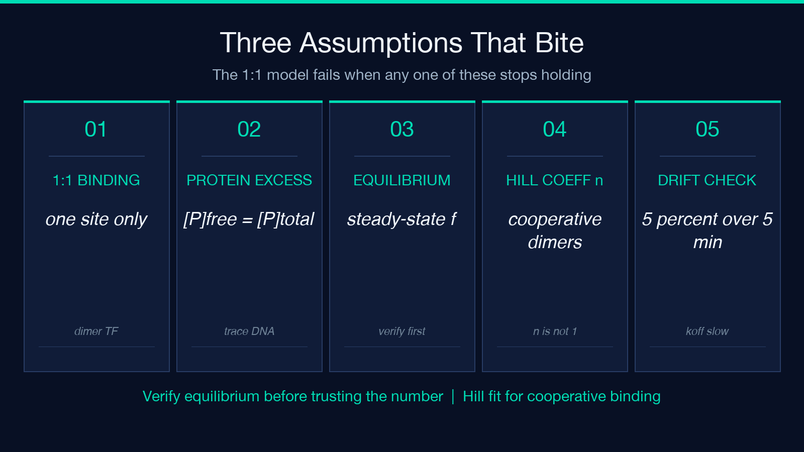
The most common real-world failure is the equilibrium assumption. A TF–site interaction with koff = 0.001 s⁻¹ has a half-life of 700 seconds, so a 10-minute incubation looks equilibrated but a 2-minute incubation does not. If your anisotropy drift is more than 5% across 5 minutes, the system is not at equilibrium and the computed Kd is wrong by a factor that depends on the missing incubation time. The calculator does not warn about this — it assumes your f value is a steady-state reading. Verify equilibrium before you trust the number.
Where the Calculator Breaks Down: Cooperative Binding, Multiple Sites, and Competitor DNA
The 1:1 model fails cleanly when the protein binds two or more sites cooperatively, when the DNA has multiple protein-binding motifs, or when competitor DNA (poly(dI-dC), salmon sperm, E. coli genomic DNA) shifts the apparent Kd by sequestering nonspecific binders. The first two cases need a Hill equation or a McGhee–von Hippel model; the third case needs a competitive binding correction. None of these are within the calculator’s scope — it is a single-point triage tool, not a full thermodynamic fitting package.
For EMSA gels with multiple shifted bands, the densitometry gives you the fraction of DNA in each band (free, single-bound, double-bound), and the calculator’s f is only valid for the single-bound band. Treat the double-bound band as a separate binding event with its own Kd and stoichiometry. For experiments with competitor DNA, the standard correction is to measure apparent Kd at several competitor concentrations and back out the specific Kd via the Cheng–Prusoff relation — well outside single-point triage but easy to do once you have the apparent Kd at three competitor levels.
The Boundary Between Triage and Publication-Grade Affinity
The single-point estimate is the right tool when you need a triage answer — “is this site specific?” — and the wrong tool when you need a publication-grade Kd with a confidence interval. The boundary is the f value’s position in the responsive band: if your measured f sits between 0.2 and 0.8, the single-point Kd is good enough for triage; if your f is outside that band, the single-point Kd has more uncertainty than the bracket from running two more points. Most published Kd values report an error bar from a full curve fit, not a single point — and reviewers increasingly ask for n ≥ 3 technical replicates.
The practical cutoff is when the answer has to defend itself. A single-point Kd suffices when the call is “this site is real, sequence-specific, sub-100 nM” and the next experiment is a ChIP-seq follow-up. A single-point Kd fails when the call has to go into a paper that will be reviewed, or when the next experiment depends on the exact Kd value (e.g., a competitor titration). The calculator does not make this call — it returns a single number regardless of how confident you can be in that number. Make the call yourself based on what the number will be used for.
When to Reach for a Full Curve Fit Instead
For publication-grade affinity, fit a full titration curve to f = [P]ⁿ/([P]ⁿ + Kd_app), extract Kd_app with error bars from the covariance matrix of the fit, and convert to ΔG° via the van’t Hoff relation. The single-point calculator handles none of that — it is a triage tool, not a fitting package. Run at least 8 protein concentrations spanning two orders of magnitude around the expected Kd, with at least 3 technical replicates per concentration.
For binding free energy decomposition — ΔH, ΔS, ΔCp — you need a full temperature sweep with van’t Hoff analysis, or better, ITC. For cooperative binding, you need a Hill fit or a McGhee–von Hippel lattice fit. For competitor DNA effects, you need a Cheng–Prusoff or direct competitor titration. The single-point calculator handles none of these, and you should not try to force it. Reach for the full curve fit the moment the answer needs to defend itself in print or in a grant aim.
Explore more tools at elysiatools.com.
