
A 100 K drop through a 5 cm steel wall does not move the same amount of heat as a 100 K drop through a 50 cm steel wall. Anyone who has sized a steam pipe, sized an insulation jacket, or watched a chilled-water line sweat through the wrong lagging knows the asymmetry is the whole point: radial conduction through a hollow cylinder is governed by a natural log, not a thickness, and the math quietly punishes the engineer who treats it like a slab. This guide walks the Cylinder Radial Heat Conduction calculator through every branch that matters: the four output bands, the four unit conversions, the three failure modes, and the four relationships between heat flow rate, heat flux, and thermal resistance. By the end you should be able to read any radial-conduction problem and predict which lever the calculator will turn first.
Why a Hollow Cylinder Is Not a Slab
The intuition that Q scales with thickness comes from the planar Fourier law, where the heat flow through a flat slab of area A and thickness t is Q = k · A · ΔT / t. For a wall whose outer surface is twice as far from the heat source as its inner surface, that intuition predicts exactly the right magnitude — but only if the area through which heat moves stays constant. In a hollow cylinder, area is not constant: it grows with radius. As heat flows outward, the same Q spreads across a larger cylindrical surface, so the radial temperature gradient decays logarithmically rather than linearly. The natural-log term ln(r2 / r1) is the integral of 1 / r from r1 to r2, which is exactly the geometry of an expanding cylinder.
That decay has a practical consequence. Adding 5 cm of insulation to a thin-walled pipe roughly doubles r2, but the log term only grows by ln(2) ≈ 0.69, not by a factor of 2. So a single 5 cm wrap reduces heat loss by about 30 percent relative to the bare pipe, not by 50 percent. The next 5 cm (from r2 = 2r1 to r2 = 3r1) reduces loss by only another 15 percent, because the same Q now has even more area to spread across. This diminishing return is why industrial lagging is sized in logarithmic increments, not linear ones, and why the calculator’s ln(r2 / r1) output is the natural axis to read along.
The Formula the Calculator Is Actually Solving
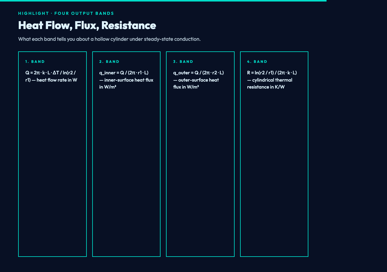
The calculator’s headline equation is the steady-state Fourier law for a hollow cylinder, written in cylindrical coordinates. For a single-layer wall with inner radius r1, outer radius r2, length L, thermal conductivity k, and temperature difference ΔT, the radial heat flow rate is:
Q = 2π · k · L · ΔT / ln(r2 / r1) (W)Three things in that line deserve attention before any number is punched in. First, the natural log ln(r2 / r1) is what turns a linear slab formula (where Q would simply be k · A · ΔT / thickness) into a radius-aware expression. Second, the geometry only enters through the ratio r2 / r1, which means doubling both radii leaves Q unchanged while doubling only r2 cuts Q roughly by the ratio of the new log to the old one. Third, the equation is positive when r2 > r1; if you swap the radii the log goes negative and so does the heat flow, which is exactly the behavior you want when the cold side sits on the outside.
The rest of the four bands fall out of Q by simple divisions:
q_inner = Q / (2π · r1 · L)          (W/m²)   inner-surface heat flux
q_outer = Q / (2π · r2 · L)          (W/m²)   outer-surface heat flux
R       = ln(r2 / r1) / (2π · k · L) (K/W)    cylindrical thermal resistance
The inner flux is always higher than the outer flux for the same Q because the inner surface area is smaller. That single ratio is what determines whether a pipe insulation strategy works: a layer that absorbs the same Q at a smaller surface has to dissipate more watts per square meter, and the inside skin temperature climbs until the inside of the lagging approaches the pipe’s outer-wall temperature.
Reading the Four Output Bands Together
The calculator returns four numbers because no single one tells the story. Heat flow rate Q answers how much energy is moving. Heat flux q_inner and q_outer answer whether the surfaces can survive that movement without exceeding a flux limit. Thermal resistance R answers how the wall behaves as a circuit element. For a layered system the resistances add like resistors in series, so the R band is the only one that lets you stack insulation, cladding, and air gaps.

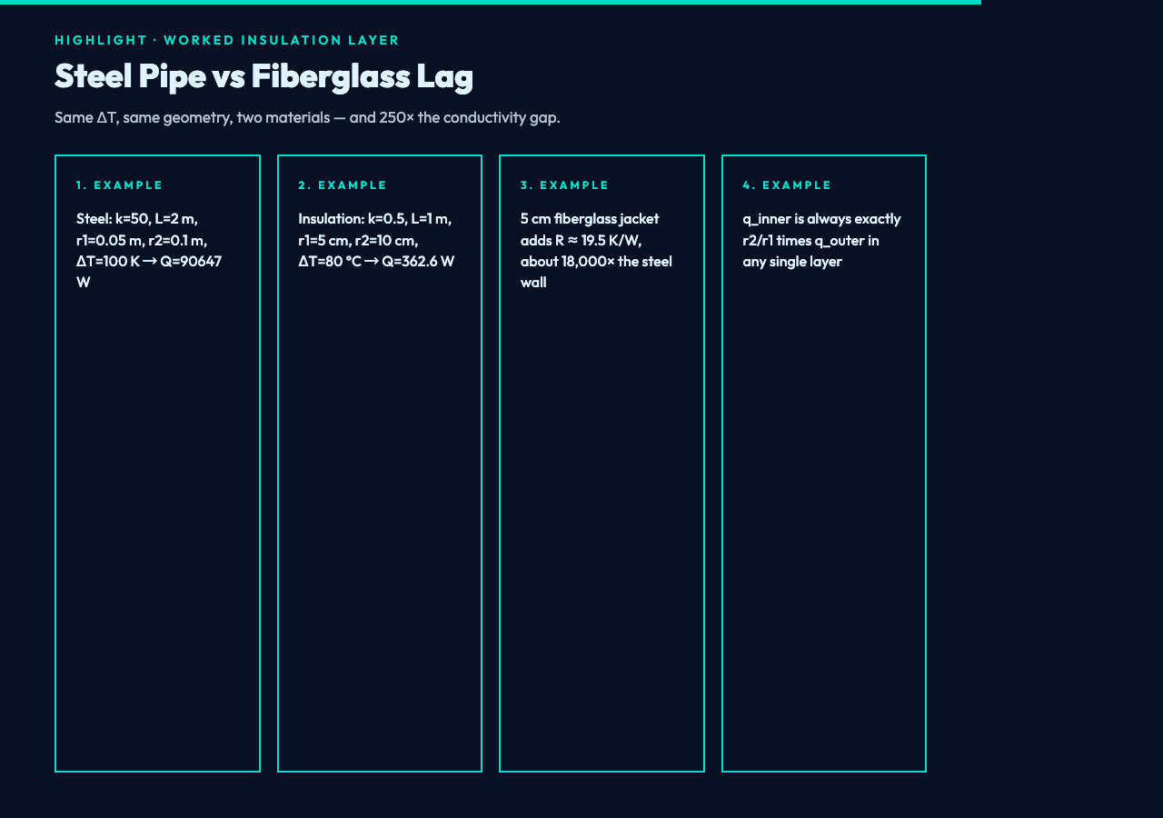
A worked example: take a steel steam pipe with k = 50 W/(m·K), L = 2 m, r1 = 0.05 m, r2 = 0.1 m, ΔT = 100 K. Plug into the calculator and the four bands come back as Q = 90647.20 W, q_inner = 144269.50 W/m², q_outer = 72134.75 W/m², R = 0.0011 K/W. The asymmetry between inner and outer flux is roughly 2:1, exactly what the radius ratio predicts. If you wrap a 5 cm fiberglass jacket around the same pipe (k ≈ 0.04 W/(m·K)), the jacket alone adds R ≈ 19.5 K/W — about 18,000 times the steel wall’s resistance — which is the engineering point of the insulation.
The Four Unit Conversions That Quietly Bite
The calculator exposes four unit selectors — length in m / cm / mm, radius in m / cm / mm, and temperature in K / °C / °F — because each conversion hides a subtle trap. Length and radius share the same scaling factor by construction (a 5 cm radius is 0.05 m either way), so the danger is input bookkeeping rather than math: feed the inner radius in cm and the outer radius in m, and the log term silently evaluates ln(0.1 / 5) = ln(0.02) = -3.91, then Q goes negative and you have to read the sign to realize the bug.
Temperature is more interesting. A ΔT in Kelvin and a ΔT in Celsius have the same magnitude (a 100 K interval is a 100 °C interval), so both units produce identical numerical results. Fahrenheit does not: a 100 °F interval is 100 × 5/9 ≈ 55.56 K. The calculator performs that conversion internally, which means if you wire the output of this calculator into a Fahrenheit-domain downstream tool without converting back, you will silently under-report the heat flow by 44 percent.
Decimal places is the fourth knob, and it is worth setting before the headline number rather than after. A 4-decimal Q value like 90647.2028 W reads as authoritative, but for a heat-loss budget on a 90 kW pipe, the last digit is dominated by k uncertainty in the steel data sheet. The 4-decimal default is honest; treating it as a precision spec is not.
The Three Failure Modes Worth Pre-checking
Three inputs can derail the calculation in ways the calculator will not catch silently.
The first is r2 ≤ r1. When the outer radius equals the inner radius the log term is ln(1) = 0 and Q divides by zero. The form will either reject the input or return Infinity depending on the path; either way, the engineer should treat the result as undefined rather than as a “no heat flows” reading. The opposite case (r2 < r1) is the cold-side-on-outside configuration and produces negative Q by design, which the form accepts.
The second is negative k or negative L. Thermal conductivity is positive for any real material, and a negative k would imply a material that pumps heat uphill. The form’s validation should reject both, but if you are feeding it programmatically, double-check the sign before trusting the output.
The third is unit-mixed inputs across length and radius selectors. Picking lengthUnit = m and radiusUnit = cm without also converting the numeric length value will silently scale one input by 100 and leave the other alone. The 18,000:1 ratio between steel and fiberglass in the worked example only holds when both inputs are in the same physical unit space.
Where the Heat Flow Is Going: A Worked Insulation Layer
Take an insulation layer with k = 0.5 W/(m·K), L = 1 m, r1 = 5 cm, r2 = 10 cm, ΔT = 80 °C (= 80 K). The calculator returns Q = 362.59 W, q_inner = 1154.16 W/m², q_outer = 577.08 W/m², R = 0.2206 K/W. Note three things. First, q_inner is exactly twice q_outer, because the inner surface area is exactly half the outer surface area in this geometry. Second, the R = 0.2206 K/W value lets you stack this layer in series with a steel pipe wall to predict the total temperature drop across a composite system. Third, the modest Q of 363 W through a 5 cm layer with a 80 K driving difference shows how badly a low-conductivity material resists heat — the steel pipe example moved 90 kW through the same ΔT with 250× the conductivity.
That order-of-magnitude comparison is what makes the four-band output valuable. If the calculator only returned Q, you would still have to compute the flux ratio by hand to know whether the lagging will burn through; if it only returned R, you would not know whether the system could actually move the heat load at all. The four outputs together let a thermal designer size the lagging, check the surface temperatures, and budget the network resistance in one pass. The Cylinder Radial Heat Conduction calculator handles the natural log and the unit conversions, but the engineering judgment — what q_inner means for the contact temperature, what R implies for the next layer in series — still lives in the chart and the engineer’s head.
Negative Delta T and Reverse Heat Flow
One branch that earns its own callout is the negative ΔT case. Setting ΔT = -50 K (or -50 °C) on the same geometry flips the sign of Q without changing its magnitude. This is the textbook behavior for a hot pipe cooling to ambient: if the engineer has set up the boundary conditions with the inside surface as the cold side, the negative heat flow simply says “heat is moving from outside in”, and the calculator returns a negative number to preserve sign consistency. Most thermal networks downstream expect a positive Q when heat moves outward and a negative Q when it moves inward; preserving the sign lets the same calculator serve both chilled-water and hot-pipe scenarios without rewriting the inputs.
A subtler branch is the magnitude of the asymmetry. The ratio q_inner / q_outer is exactly r2 / r1 for any single-layer wall, regardless of k, L, or ΔT. So a 2:1 radius ratio always produces a 2:1 flux ratio. That invariant is useful for sanity-checking the result: if the calculator reports a flux ratio of 1.7 against a 2:1 geometry, the most likely cause is a unit mismatch on one of the radii, not a bug in the calculator.
When the Cylinder Approximation Breaks Down
The radial-conduction formula assumes an infinitely long cylinder with end effects ignored. For a short pipe stub — say, a 5 cm long cylinder attached to a much larger tank — the end surfaces carry a non-trivial fraction of the total heat flow, and the 2D heat-transfer problem has to be solved with shape factors from conduction shape-factor tables. The calculator’s input form asks for L precisely so the user can decide whether the cylinder is long enough for the approximation to hold. A safe rule of thumb is L > 5 × r2; below that, the radial-only assumption underestimates the total heat flow by 10–20 percent.
The second breakdown is anisotropic material. The formula assumes k is the same in every direction. For woven insulation or layered composites, the conductivity parallel to the fibers is much higher than perpendicular, and the calculator’s single k input averages them in a way that no real geometry respects. For those materials, the engineering answer is to use the perpendicular k for radial conduction and account for the parallel path with a separate fin model.
For other thermal regimes worth comparing against this radial model, the heat-conduction calculator, the heat-convection calculator, and the heat-radiation calculator cover the planar, fluid, and radiative branches respectively. Explore the broader library at elysiatools.com/en/tools.
