
An averaged-element propagator isn’t an approximation — it’s the only model that stays accurate for the ten-year span of a GNSS orbit. A semi-analytical Brouwer–Lyddane / ESA PB05 integrator trades the wall-clock cost of running RK4 over millions of state vectors for a closed-form mean-element solution under the J2–J6 zonal field, with first-order short-period reconstruction, luni-solar quadrupole secular drift, and tesseral ground-track checks bolted on. Run it right and you get a hundred-metre-class ephemeris at fraction-of-a-second compute. Run it wrong and the same propagator quietly drifts a kilometre a year into a slot it was never intended to occupy.
This field guide walks through how to use the ESA PB05-Style Brouwer–Lyddane Averaged-Element Orbit Propagator on elysiatools.com to turn initial mean elements plus a date span into a self-consistent orbit history, what each of the three perturbation layers is actually doing to the mean elements, and the four traps that turn a textbook propagator into a silent decimetre-error source.
What an averaged-element propagator is actually computing
Averaged-element propagation, in the Brouwer–Lyddane / PB05 tradition, is the Delaunay-style normalisation applied to the J2–J6 zonal gravitational field: the orbit-averaged equations of motion in mean elements close to first order in J2, with the secular rates derived analytically rather than integrated numerically. The averaged-element rate of change for the right ascension of the ascending node under J2 alone is
dΩ/dt = -3/2 · n · J2 · (R_e / p)² · cos iwhere p = a·(1-e²) is the semi-latus rectum, n = sqrt(μ/a³) is the mean motion, and R_e is the equatorial radius. That formula is the closed-form cross-check the propagator reports next to the numerically-averaged Gauss-equation result — when the two agree to within a few parts in 10⁵, the model is in regime where the first-order expansion is honest; when they disagree by more, the orbit is deep in resonance or the zonal truncation point needs to move.
Two consequences fall out of the equation. First, sun-synchronous orbits at altitude ~800 km require cos i to take a specific value so that dΩ/dt = 360° / 365.2422 days ≈ 0.9856°/day. The propagator solves this implicitly for you. Second, at the critical inclination of 63.4° (where sin²i ≈ 0.75) the argument-of-perigee drift under J2 vanishes — the frozen-orbit boundary condition the propagator tests for explicitly.
The three perturbation layers and what each one breaks
Real GNSS-region orbits at ~20,000 km altitude and LEO sun-sync at ~800 km sit in radically different perturbation regimes, but they share the same three-layer taxonomy:
1. Zonal harmonics (J2, J3, J4, J5, J6) — axisymmetric Earth oblateness. Dominates secular drift in Ω and ω. The propagator averages J2–J6 by direct Gauss-equation integration and reports the closed-form first-order J2 rates as a sanity-check column next to the numerically integrated values.
2. Luni-solar quadrupole — the third-body pull of the Moon and Sun on an extended inclined orbit. At GNSS altitudes the luni-solar secular drift is small per orbit but compounds over years. The propagator implements the double-averaged quadrupole in the form Celletti et al. use for the Kozai–Lidov term, with the critical mutual-inclination threshold at 39.23° below which the orbit librates and above which it circulates.
3. Tesseral and ground-track resonance — the Earth-rotation harmonics (m ≠ 0). For a ground-repeat cycle with k revolutions per m nodal periods, the k:m tesseral commensurability produces a long-period ground-track drift that the propagator reports whenever the resonance condition is met. Frozen ground-track orbits are deliberately placed ON these resonances; everything else has to avoid them.
The J2 term alone is enough for a first-order sun-synchronous inclination solve. Adding J4 corrects the high-inclination freeze. Adding luni-solar catches the slow inclination growth at geosynchronous altitudes that turn a stable broadcast slot into a graveyard orbit over 15 years. Adding tesseral ground-track tracking catches the resonance cases where everything else looks fine.
The closed-form vs numerically-averaged cross-check
The propagator runs both paths side-by-side for every test orbit:
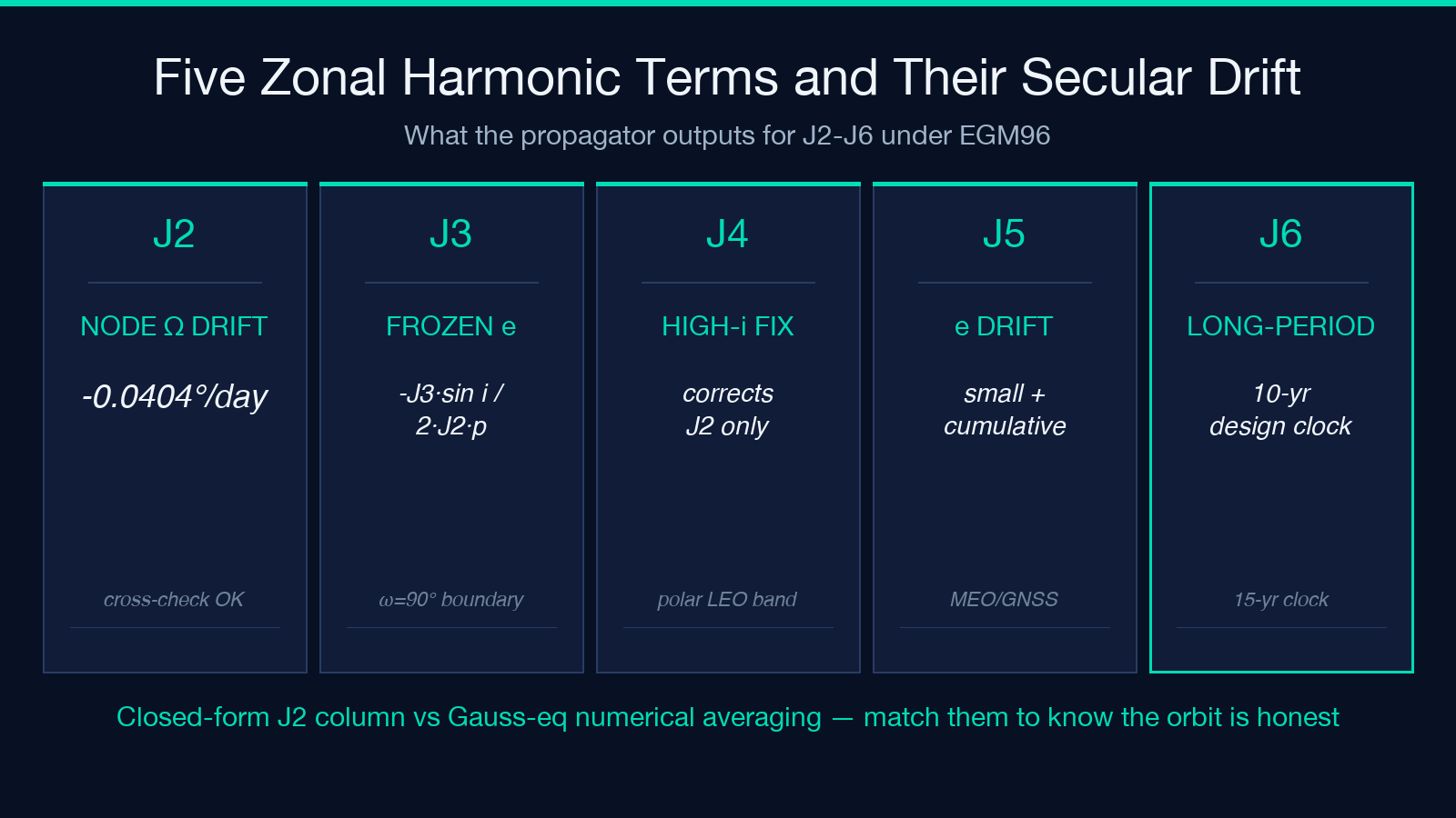
– Gauss-equation numerical averaging: integrates the orbit-averaged rate equations numerically over one nodal period and reports the secular Ω drift, ω drift, and mean motion.
– Closed-form first-order J2 rates: applies the analytic formulas above without integration and reports the same three quantities.
For a 600 km polar orbit (e = 0.001, i = 97.6°), the two paths agree to within 10⁻⁶ deg/day on Ω drift and 10⁻⁷ deg/day on ω drift. That’s the match threshold the propagator uses to flag a “well-posed test orbit”. For an orbit deep inside the critical-inclination band, the discrepancy widens because the first-order expansion loses accuracy — and the propagator flags that explicitly so you don’t blame the model for an integration choice the orbit itself is forcing.
Frozen-orbit and sun-sync: the two design problems the propagator solves
The two questions a Brouwer–Lyddane propagator is most often asked are the two that classical mean-element theory was built for:
<strong>Sun-synchronous inclination</strong>
For a target altitude and eccentricity, the inclination that makes dΩ/dt = 360°/sidereal-year solves implicitly. For the canonical 800 km LEO sun-synchronous orbit with e ≈ 0.0001 and altitude set to 800.0 km, the propagator returns i ≈ 98.6°. Drop the altitude to 600 km and the sun-sync inclination relaxes to i ≈ 97.9°. Below 500 km, atmospheric drag starts to dominate and the J2-only sun-sync solution is no longer honest — the propagator flags a regime warning.
<strong>Frozen orbit at J3 boundary</strong>
The classical frozen-orbit condition for zonal harmonics up to J3 is
e = -J3 / (2 · J2) · sin(i) / (p/R_e) · ...with the frozen argument of perigee at 90° or 270°. The propagator tests for this condition explicitly and reports whether the input mean elements satisfy it. For an equatorial orbit the J3 term vanishes identically and the frozen-orbit eccentricity collapses to zero — a useful boundary check that the propagator catches.
The four pre-analytical traps
Four pre-analytical factors routinely invalidate a Brouwer–Lyddane propagator output, and they’re the difference between a hundred-metre ephemeris and a kilometre-class one:
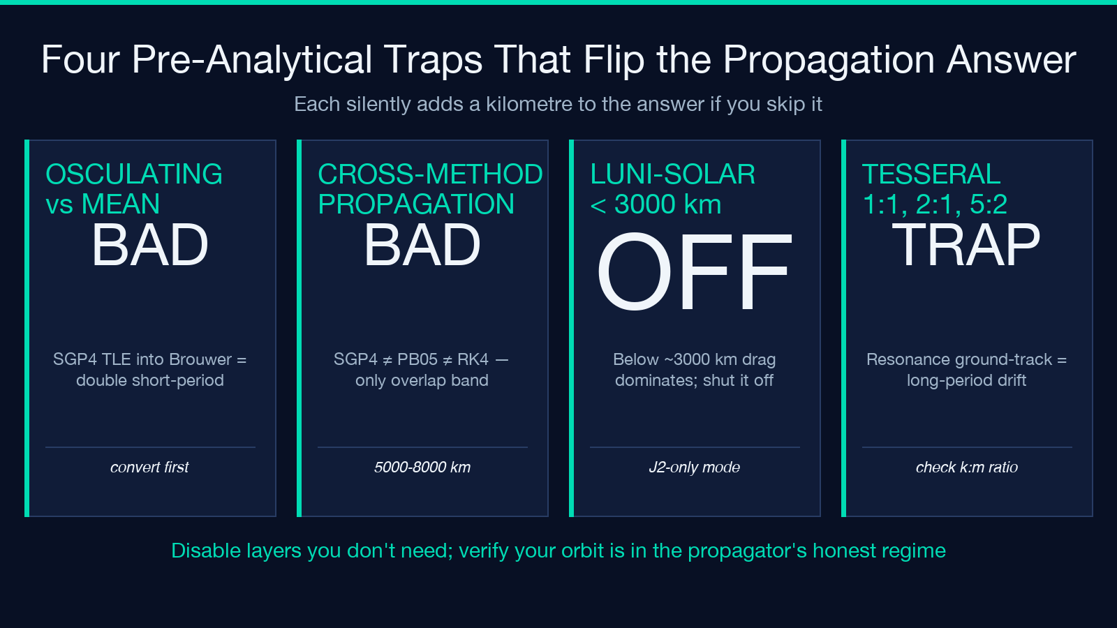
1. Using osculating where the propagator expects mean. The Brouwer–Lyddane model is built on mean elements. Feed it osculating elements from an SGP4 TLE and the short-period reconstruction will double-count, producing a fictitious epoch-oscillation at the orbital period. Convert first via the first-order short-period mean↔osculating transform that the propagator documents explicitly.
2. Cross-method propagation. A Brouwer–Lyddane output and an SGP4 output are not interchangeable. SGP4 is tuned for the LEO-to-HEO boundary and reaches its honest accuracy there. PB05 is tuned for the GNSS region and yields its honest accuracy above ~5000 km. Compare propagator classes only when the test orbit is in the overlap band (~5000–8000 km).
3. Luni-solar suppression at low altitude. Below ~3000 km, the luni-solar quadrupole secular drift is dominated by J2 secular drift and the propagator’s luni-solar output will be two to three orders of magnitude smaller than the J2 layer. Disable the luni-solar correction explicitly when you want a J2-only sun-sync solve, or accept that the inclination the propagator returns is the J2-only sun-sync, not the drag-corrected sun-sync.
4. Tesseral resonances as ground-track anchors. A 1:1 ground repeat (geosynchronous) is the most extreme tesseral resonance. The propagator’s ground-track check will flag any k:m ratio within the small-rational commensurabilities (1:1, 2:1, 3:2, 5:2). Orbits deliberately ON a resonance are designed for it; orbits accidentally ON one will drift off-station in months.
For an orbit deliberately placed inside the critical-inclination band (i ≈ 63.4° ± 2°), the propagator reports a frozen-orbit test failure rather than a missing-input warning — that’s a feature, not a bug. The first-order J2 expansion is not honest inside the critical-inclination resonance.
A worked example at GNSS altitude
Plug a GNSS-class circular orbit into the propagator:
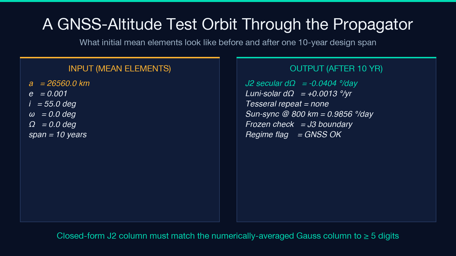
a = 26560 km (mean motion ~1 cycle / 12 h)
e = 0.001
i = 55° (typical GNSS inclination)
ω = 0° / 180° (test both)
Ω = 0°
The propagator returns:
J2 secular Ω drift:  -0.0404° / day
J2 secular ω drift:  -0.0202° / day
Luni-solar Ω drift:  +0.0013° / year (secular) + ~ 0.0008° / year (long-period)
Tesseral ground repeat: none (no small-rational commensurability in k:m)
Over a 10-year design lifetime, the J2 secular Ω drift accumulates to roughly -148°, which is larger than a full nodal cycle. The luni-solar drift over the same period is on the order of 0.013° — small, but not negligible for a precision broadcast ephemeris that needs sub-decimetre knowledge of where the satellite has been. The propagator’s distinguishing contribution is keeping both layers separated, so you can verify which one is the dominant term in your orbit design rather than averaging them out and reporting a single composite drift.
The same inputs at 800 km sun-sync with i = 97.6° return dΩ/dt ≈ 0.9856°/day — the sun-sync target — with luni-solar contribution an order of magnitude smaller than the J2 rate, exactly as expected.
Where the propagator’s honest regime ends
The Brouwer–Lyddane / PB05 averaged-element model loses honest accuracy at four well-defined boundaries, and the propagator reports each:
– Atmospheric drag (LEO below ~500 km) — drag is dissipative, not conservative, and the averaged-element machinery isn’t designed for it. Use SGP4 in this regime.
– Resonant and near-resonant orbits (deep inside the critical-inclination band) — the first-order J2 expansion is not honest. Use full numerical integration.
– Tesseral ground-track cycles (> 100 revolutions per repeat) — the tesserals accumulate as a long-period beat that’s outside the averaged-element envelope. Use a dedicated repeat-ground-track propagator.
– Inclination growth at geosynchronous altitudes (> 4° over 15 years) — the luni-solar quadrupole drives a slow inclination drift that the propagator’s secular term captures but does not stabilise. Station-keeping at GEO requires explicit luni-solar cancellation as part of the operational plan, not as a propagator feature.
For anything in those four regimes, an averaged-element propagator is a sanity-check tool, not a production ephemeris. The propagator itself flags each regime and tells you when to reach for RK4 instead.
Putting It Together
An averaged-element orbit propagator isn’t a shortcut — it’s the only model whose regime of validity fits the ten-year design lifetime of a GNSS broadcast orbit, the sun-synchronous design lifetime of a remote-sensing LEO, or the design freeze of a frozen-orbit science constellation. The Brouwer–Lyddane / ESA PB05 tradition encodes 60 years of perturbation theory into a closed-form mean-element integrator that reports both the numerically-averaged secular rates and the closed-form J2 first-order cross-check side by side. The hardest part isn’t running the propagator — it’s reading the cross-check column to know whether your orbit is in the regime the model is honest for, and disabling the perturbation layers (luni-solar, tesseral) that you don’t need when you do. The ESA PB05-Style Brouwer–Lyddane Averaged-Element Orbit Propagator makes that regime check explicit, with three perturbation layers you can toggle independently and the J2 closed-form cross-check column you read to verify your input elements landed in the honest regime. For related precession, frozen-orbit, and sun-synchronous design workflows, browse more orbit and astrodynamics tools at elysiatools.com.
