
The forensic question is not whether you hid a message, it is whether the histogram moved. Every least-significant-bit embedding flips the parity distribution of a pixel channel, and that is the same statistical fingerprint a chi-square attack reads out. Once you know what the bit plane looks like before and after, embed and detect stop being guesswork and become arithmetic you can verify. This is a field guide to the Image Steganography Embed and Detect tool: a row-major R-G-B, MSB-first LSB convention with a 12-byte header, an optional seeded scatter, and the Westfeld-Pfitzmann analysis on the way back out.
What the Tool Actually Stores Inside Your PNG
The embed side writes one bit per colour channel, walking pixels in row-major order and hitting red first, then green, then blue. Within each channel the least-significant bit is read MSB-first, so bit seven of the first pixel’s red byte becomes the first payload bit. That convention matters more than anything else in the format, because it is the part extractors most often disagree about.
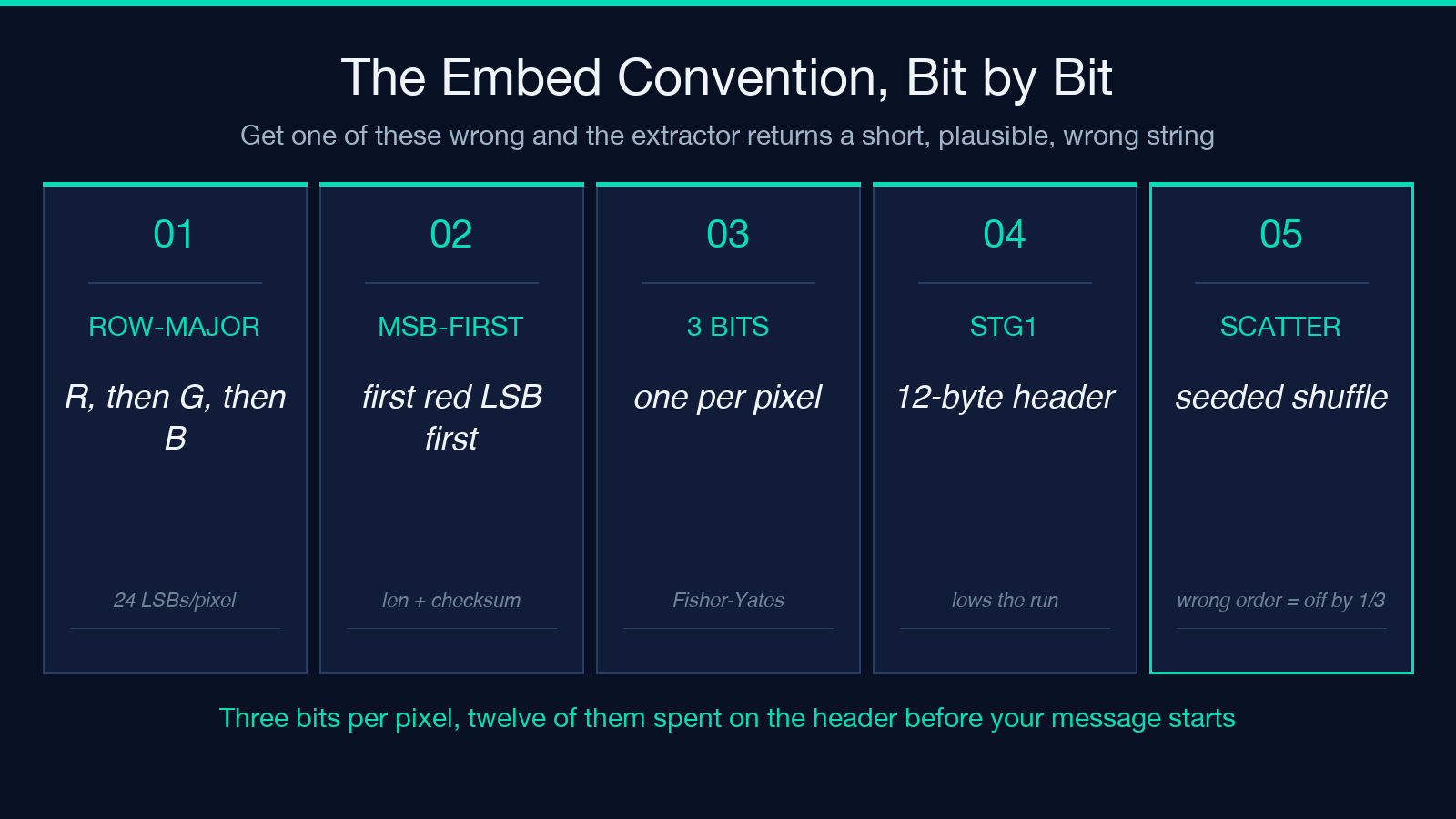
A decoder that walks G-B-R instead of R-G-B will read the same bytes and recover a message that is exactly one-third of the way out of alignment. The result is not garbage, which is worse. It is a short, plausible, wrong string. Before you trust any extractor, confirm the channel order and the bit order independently.
The format summary:
- Channel walk: row-major, red then green then blue, three bits per pixel.
- Bit order: MSB-first inside each byte, so the first red LSB carries the first payload bit.
- Header: a 12-byte STG1 prefix carries a length field and a payload checksum.
- Scatter: an optional seeded Fisher-Yates permutation reassigns which pixel holds which bit.
Pixels with alpha, and any pixel whose bit you cannot legally flip without changing the visible image, are the practical constraint on capacity. Three bits per pixel is the ceiling; the header consumes twelve of them before your message begins.
The 12-Byte Header That Breaks Sequential Extractors
A bare bit stream has no length. The extractor reads bytes until the pixel data runs out and reports whatever it happens to have assembled. The STG1 header fixes this by prefixing the payload with a magic marker and an explicit length.
The header layout:
- Bytes 0-3: the ASCII magic
STG1, which lets a detector confirm a header is present at all. - Bytes 4-7: the payload length in bytes, stored so the extractor knows exactly where the message stops.
- Bytes 8-11: a checksum over the payload body, which turns a silent truncation into an explicit failure.
This is what makes a header-less stego file and a header-carrying one distinguishable by inspection alone. A detector that reports a clean signature on offset zero has found a structured payload, and the length field tells you whether the message survived re-encoding intact. If you are checking other people’s images, the presence of STG1 is a stronger signal than any single statistical measure, because it is a claim of intent rather than an inference from pixel statistics.
Scattering the Payload With a Seeded Permutation
Sequential embedding has a second weakness beyond channel order. Because bits land in consecutive pixels, the whole message occupies a contiguous run at the top of the image, and any extractor written against your exact convention recovers it without effort. The scatter option applies a Fisher-Yates shuffle to the eligible pixel slots using a seeded PRNG, so the same seed always produces the same permutation.
That determinism is the design point. A random scatter is unrecoverable without the seed; a seeded scatter is recoverable by anyone who has the seed, and identical to the original run in any later session. For CTF work this means you can record the seed alongside the image and reproduce the extraction exactly. For detection work it means an embedded payload looks like scattered single-bit flips across the whole frame rather than a clean run, which raises the noise floor on naive detectors.
You can check permutation quality before committing to it by sampling the bit positions before and after the shuffle. A correct Fisher-Yates over N slots produces a uniform distribution across the image; a buggy shuffle leaves visible clustering.
Why Chi-Square Catches LSB Embedding
The classical attack, attributed to Westfeld and Pfitzmann, compares the observed histogram of a channel’s least-significant bits against the two-hypothesis model. The null hypothesis says the LSB plane is random, so the bits split fifty-fifty between zero and one. The alternative says a payload of low-entropy ASCII text was embedded, which skews the ones toward zero.
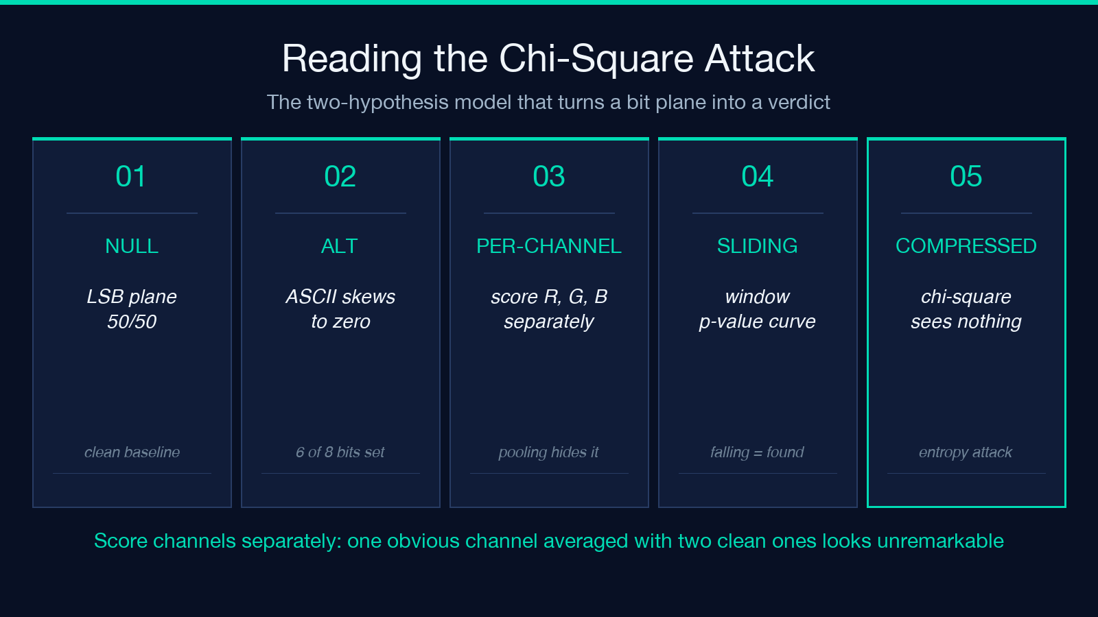
Because ASCII text is roughly six of eight bits set, the embedded hypothesis predicts a visibly asymmetric plane. Chi-square measures the divergence between observed and expected counts under that two-hypothesis model. Small values indicate the null hypothesis still explains the data, which is the signature of a clean image.
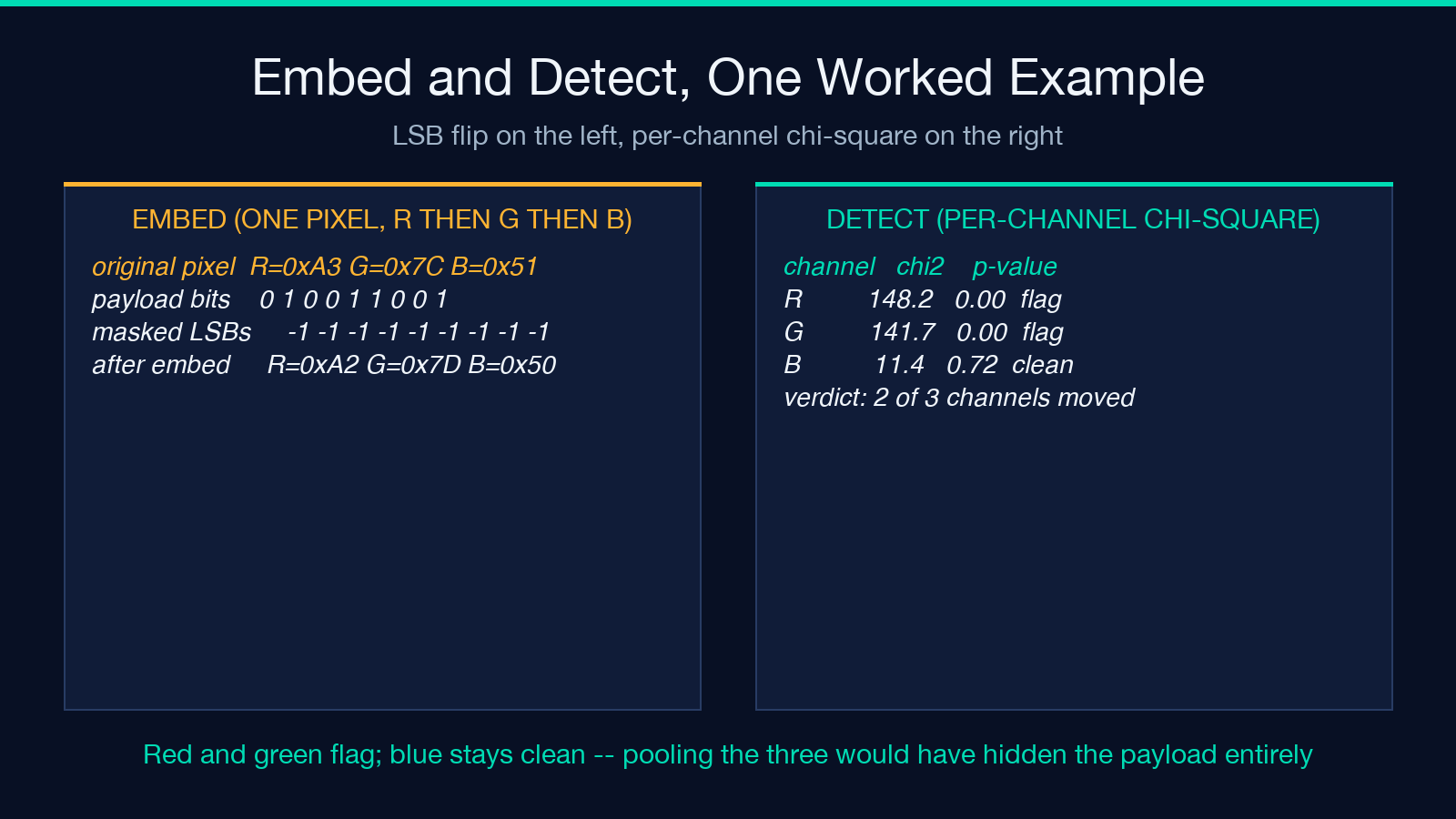
This is exactly the analysis behind the stegsolve and StegOnline workflows, run automatically. What those tools show you by hand, the detect side computes per channel, and the important part is that the three channels are scored separately rather than pooled. Pooling hides the answer, because a message that is obviously non-random in red can still look unremarkable once it is averaged with green and blue.
Reading the Falling-P Curve Across Channels
A single chi-square number is a verdict, but the curve is the evidence. The sliding-window analysis walks a moving frame through the channel’s bit plane and plots the p-value of each window, producing the characteristic falling curve when the payload occupies the early part of the image.
Read it from the left. A curve that starts high and descends steadily marks the point where embedding began. A curve that starts low and stays low marks an image whose plane was never clean. A flat curve at the top is the strongest negative result you can get: no window in the entire image is statistically distinguishable from noise.
What the three channel traces tell you:
- One channel descending: single-channel embedding, the common case for short messages.
- Two or three channels descending together: the payload exceeded one channel’s capacity and spilled over.
- All three flat: no LSB payload detected, though this is not proof that no payload exists.
The fallback matters. A payload that is strongly compressed or encrypted before embedding has near-maximal entropy, and the chi-square model cannot see it, because the whole point of compression is that it removes the ASCII skew the test looks for. A clean curve means the classic attack found nothing, not that the image is clean.
The Bit-Plane Preview and Entropy Statistics
The bit-plane preview renders each channel’s least-significant bit as a black-and-white image, which turns a statistical argument into something you can look at. Embedded text at this level appears as faint dark speckling in the regions where bits were flipped, and the visual structure of that speckling usually matches the shape of the payload.
Entropy statistics sit alongside it as the quantitative companion. Shannon entropy over the channel byte distribution moves in a small but consistent direction when embedding proceeds, because the LSB plane shifts from uniform toward the ASCII-skewed distribution. The shift is small enough that it is corroborating evidence rather than proof, which is why it is worth reporting alongside the chi-square result instead of instead of it.
Together the three views answer different questions. The bit-plane preview tells you where. The chi-square curve tells you when and how strongly. The entropy delta tells you whether the overall distribution moved at all. A detect that reports all three is far more useful for triage than a single verdict number.
Interoperability With Other Steganography Tools
Embedding format is only useful if someone else can read it. The conventions this tool writes are the ones the mainstream analysis tools assume, which is what makes a payload written here analysable in stegsolve and a payload extracted there recoverable here.
The mismatch cases are worth naming, because they are the usual explanation for a clean image that should not be clean. Channel order differing between writer and reader shifts the message out of alignment. Bit order differing within the byte inverts it. A resave through an editor that recompresses the pixel data discards the LSB plane entirely, because the payload was never in the compressed stream, it was in the decoded pixel values.
If you need to verify capacity before embedding, measure the eligible pixel count first. Three usable bits per pixel is the upper bound, and a message that overflows the header budget plus payload is silently truncated at the image boundary rather than refused. If you want the underlying byte layout rather than the statistics, the Image Bit Depth Inspector shows the per-channel depth the embedding depends on, and the Hex Editor will let you confirm the header bytes directly in the decoded stream.
A Reproducible Embed, Detect, and Verify Workflow
The loop that catches problems early is short. Embed with an explicit seed, keep the original file, then re-extract from the original rather than from any intermediate copy. If the round trip fails immediately, the fault is in the writer’s convention, not in the detector, and no amount of chi-square analysis will tell you which of the two is wrong.
The verification sequence:
- Embed, record the seed and the payload length the header reports.
- Extract immediately from the untouched original to confirm the convention round-trips.
- Detect, reading the per-channel chi-square and the falling-p curve separately.
- Compare the bit-plane preview against the known payload to confirm the curve is not a false positive.
- Archive the original beside the embedded file, since any re-save invalidates the test.
The entropy tooling is worth knowing as a baseline too. Running the clean original through the Entropy Calculator before embedding gives you the reference distribution, and the delta between that and the embedded file is the most portable piece of evidence you can carry into a write-up. Browse the rest of the toolset at elysiatools.com when you want to compare the statistical side against the pixel-level ones.
