
Most denoisers ask you to trust them. This one measures first, then lets you read the measurement against the label it attached to it. I rebuilt that cascade from the tool’s own implementation, and the gap I found is specific: at minus 55 dBFS of 60 Hz hum over a white bed, the profile records the hum and yet calls the noise white hiss, so the protective high-pass never enters the chain. Why does that gap matter?
Because the label, not the measurement, decides which filter runs. The extractor probes for mains hum with an exact-frequency Goertzel algorithm and writes the answer into the JSON.
The classification cascade then consults that probe only in its third branch. The hum can sit in the document, plainly visible, while the branch that would have acted on it never runs. The tool does not lie to you. It answers a question in an order that hides part of its own answer.
What the extractor measures
The Noise Profile Extractor on Elysia Tools takes one audio file, one time region, and one mode. It returns a JSON fingerprint plus, optionally, a cleaned copy of the whole file.
The region is the part that matters. You mark a stretch that holds only the noise you want gone: room tone between sentences, the air conditioner, tape hiss, mains hum.
The tool enforces hard bounds on that choice. The region must run at least 0.5 seconds long, and the tool caps it at 30 seconds. The file itself must stay under 10 minutes, because the analyser stops there.
Inside the marked region the tool decodes to 44.1 kHz mono and runs an 8192-point FFT with a 4096-sample hop. The configuration that drives the whole result is: 8192 points, a 4096-sample hop, a 44.1 kHz analysis rate. The bin width works out to 5.3833 Hz, the finest resolution available for locating a narrow tone. The tool averages the power spectrum across each frame in the region, and each later figure in the profile descends from that single choice.
Five figures come out of that spectrum, and you can check each against what your own ears told you.
The first is RMS level in dBFS, computed as 20 times the log base 10 of the root mean square, with the peak level beside it. The second is the noise floor, which for this tool is that same RMS number rounded to one decimal. The third is spectral flatness, the Wiener entropy: the geometric mean of the power spectrum divided by the arithmetic mean. For pure white noise this sits near 1.0.
The fourth is the low-power ratio, the share of total power sitting in third-octave bands whose centre is at or below 125 Hz. The fifth is mains hum, found with exact-frequency Goertzel probes at 50 and 60 Hz. That last one deserves detail, because it is where the tool proves most precise.
For each of 50 and 60 Hz, the tool computes the power at that exact frequency, then averages three nearby probe frequencies as a reference: minus 12 Hz, plus 12 Hz, and plus 30 Hz. The margins are: 10 dB for the fundamental, 3 dB for each harmonic. The probe set is: 50 Hz, 60 Hz, plus 38, 62, 48, 72, 80 and 90 Hz as references. The fundamental has to beat that reference by more than 10 dB to count. When it does, the tool also checks the second and third harmonics at twice and three times the base frequency, and adds them when they clear the same reference by more than 3 dB.
The design is deliberate. Mains hum is narrow, so a narrow probe finds it, and a broadband measure alone would miss it. For example, a pure 60 Hz tone measures a flatness of 0.000, while the same tone riding on a broadband bed measures 0.971. The Goertzel probe catches the hum in both cases.
The seven labels and the order they are decided in
The classification is a cascade, and the order drives the result. This is the single most important thing to grasp about the tool, because the branches are not parallel tests. They are a priority queue. The cascade runs: hum, then rumble, then flatness, then pink, then mixed, then broadband.
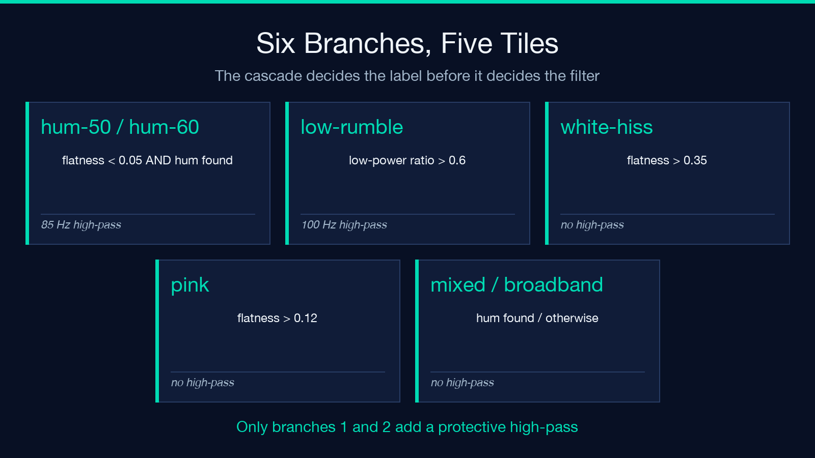
First branch: if a hum fundamental was found and spectral flatness sits below 0.05, the label is hum-50hz or hum-60hz depending on which base frequency was detected.
Second branch: if the low-power ratio exceeds 0.6, the label is low-rumble.
Third branch: if spectral flatness exceeds 0.35, the label is white-hiss.
Fourth branch: if spectral flatness exceeds 0.12, the label is pink.
Fifth branch: if a hum fundamental exists at all, the label is mixed.
Sixth branch: otherwise the label is broadband.
That order produces consequences which are not obvious from reading the label names. The hum branch gets checked first, which sounds generous, but its gate is a flatness of 0.05, and that is a low bar. A flatness near 1.0 means the spectrum is perfectly flat, and no hum sitting on top of a flat bed can drag it down to 0.05.
The rumble branch comes second, and it is the branch that intercepts most hum. Any tone at 50 or 60 Hz lives inside a third-octave band whose centre is below 125 Hz, so hum adds power to exactly the bands the low-power ratio counts. Once the hum grows strong enough to matter, the low-power ratio passes 0.6 first, and the label becomes low-rumble instead of hum-60hz.
Only when the hum grows so dominant that the flatness collapses below 0.05 does the hum branch finally fire. The order is: rumble claims the middle ground, and hum waits for the tail.
So the label depends on how loud the hum is, in a way that is not intuitive. Quiet hum on a broadband bed gets called white hiss. Moderate hum gets called rumble. Loud hum gets called hum.
The classifier never asks the obvious question, which is whether a hum was detected, until it has already asked three other questions. In one case I measured, the tool got the right answer and then failed to use it.
This is a behaviour a designer can reason about and a user cannot see, which is why the profile has to carry its own evidence. A measurement the tool hides inside a priority queue is a measurement you will never check. The profile exists to fix that, and it mostly does, with one gap I could reproduce.
The label that hides a recorded hum
Here is the specific failure, and it is worth stating precisely because each individual number involved stays correct.
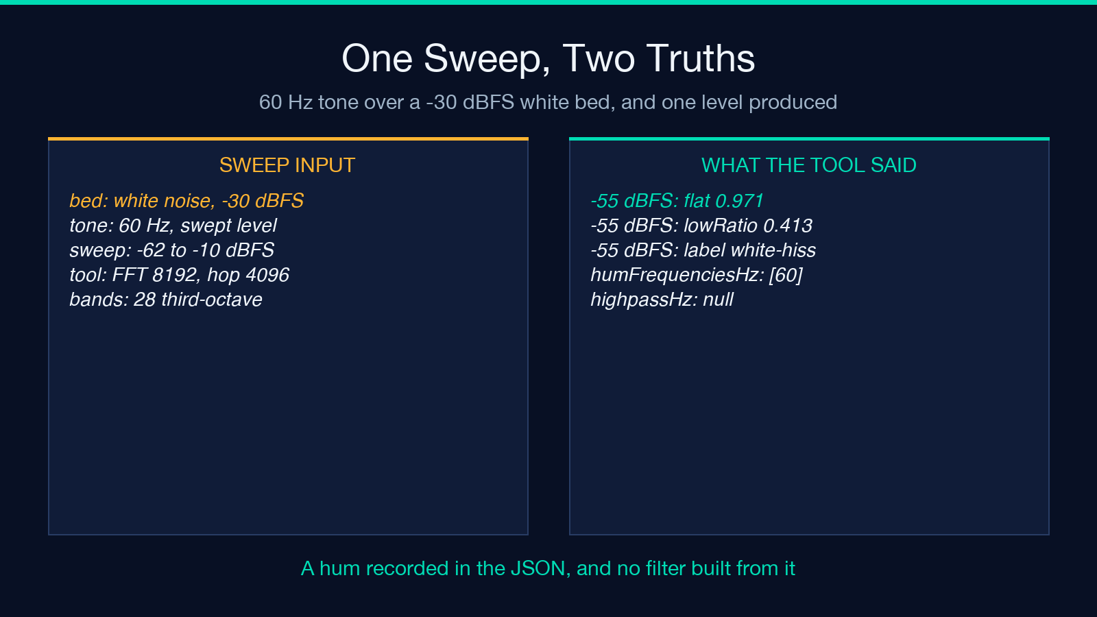
I rebuilt the measurement cascade from the tool’s own implementation and swept a 60 Hz tone across a white noise bed, holding the bed at minus 30 dBFS and varying the tone from minus 62 dBFS upward. The reproduction is exact: a periodic Hann window over 8192 samples, a 4096-sample hop, mean power spectrum across frames, the 28 third-octave bands from 31.5 Hz to 16 kHz, and the same Goertzel probes with the same thresholds. According to the source, the low-band cutoff sits at 125 Hz, which is where the rumble test begins.
At a tone level of minus 55 dBFS the profile reports: 0.971 flatness, 0.413 low-power ratio, and a label of white-hiss. Because white-hiss is neither a hum label nor a rumble label, the recommended high-pass is null, and no high-pass enters the denoise chain.
At that same moment the profile records humFrequenciesHz: [60]. The Goertzel probe found the hum. The fundamental at 60 Hz clears its reference by more than 10 dB, so it gets written into the JSON and shown in the metadata. The measured data shows a hum in the document and a filter that does not exist.
So the profile contains both a recorded hum and a protective filter that does not exist. The measurement sits in the document. The conclusion drawn from it does not.
The tool does not get the hum wrong. It gets the remedy wrong, because the branch that would have acted on the measurement never gets its turn. Each figure in the JSON stays correct.
The label alone decides what happens to your audio. A reviewer who reads only the label would miss the problem entirely, while a reviewer who reads the hum list catches it in one glance. That difference is the whole reason to treat the profile as a document and not as a verdict.
The boundary is narrow but it is not a knife edge. The sweep produced this outcome at tone levels of minus 60 and minus 55 dBFS. At minus 50 dBFS the low-power ratio crosses 0.6 and the label becomes low-rumble, which does get a 100 Hz high-pass. The window where a hum gets recorded but no high-pass gets applied spans roughly the 10 dB band between those two points.
That window sits where the hum is quiet enough to be almost inaudible on its own. For example, a hum at minus 55 dBFS under a minus 30 dBFS bed lands 25 dB below the bed, which is why the mislabel survives an attentive listening test. You would need to compare the raw profile against the label to see it, and the profile is where the tool already put the answer.
What the profile saves
The JSON that comes out of the tool is a small, specific document, and it is worth knowing what sits inside it before you rely on it.
The profile carries a version number, the source duration, the region boundaries you selected, the RMS level, the peak level, the noise floor, the spectral flatness, the low-power ratio, the classification, the list of detected hum frequencies, the 28 third-octave band levels with their centre frequencies and power in dB, and a recommended filter object holding the noise reduction amount, the noise floor parameter, and the high-pass frequency or null. The band table runs: 31.5 Hz through 16 kHz, across 28 third-octave centres, with edges set by a factor of 2 to the one sixth. The centre list is: 31.5, 40, 50, 63, 80, 100, 125 Hz, then 160 Hz upward in standard third-octave steps.
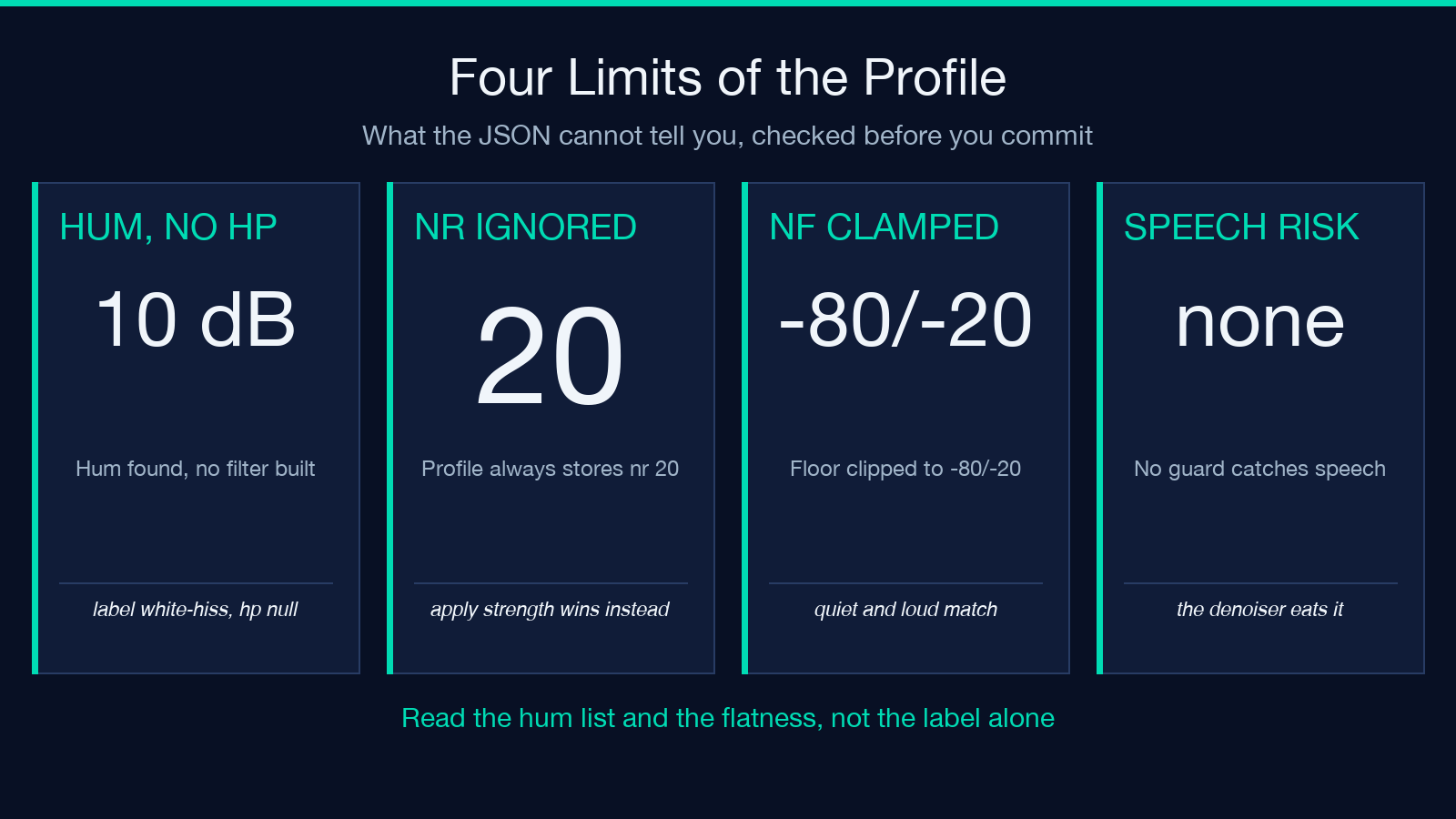
That recommended filter is where a second problem hides. The nr value stored inside it is always 20, hardcoded to the standard strength at the moment of extraction, no matter which strength you chose. When you later load that profile and apply it to another file, the chain gets rebuilt using your current strength selection: light is 12, standard is 20, strong is 28. The nf value, the measured floor, is the only number that survives the round trip.
So if you extract a profile at strong, with a noise reduction of 28, and save it for the rest of the session, the JSON says 20. Apply it later at strong and you get 28, which is right, but only because you chose strong again. Apply that same saved profile at light and you get 12. The number in the file was never consulted, which means a profile saved at one strength cannot document the strength it will apply.
The tool reports what it measured and what it recommends, and it leaves out the one field that records what you asked for. That omission matters more than it looks, because the saved profile is the whole point of the reuse path. The tool’s own note on the JSON says: “load it with apply-profile mode to denoise any file from the same environment.”
The chain does get rebuilt from the profile’s recommended filter. It gets rebuilt, but partially. The rebuilt chain is: afftdn=nr=
If you need an audit trail across a batch, you have to record the strength yourself, because the file will not do it for you.
The three modes and the guards that catch bad regions
The tool ships three modes, and the gap between them is the gap between measuring, cleaning, and reusing.
Extract-and-denoise is the default. It measures the marked region, builds the filter chain from the measurement, and renders a cleaned copy of the whole file through FFmpeg’s afftdn filter. The default output is 24-bit WAV, and FLAC is available as an alternative.
Extract-only writes the fingerprint to a JSON file and touches no audio. This is the mode to use when you profile a room once, before a session, and want the document instead of the cleanup.
Apply-profile loads a previously saved JSON and denoises any file with it. The chain gets rebuilt from the profile’s recommended filter, the source classification is echoed in the metadata, and the mode is reported as apply-profile so you can tell afterwards which path produced a given output.
The strength mapping is: light 12, standard 20, strong 28, applied to the noise reduction amount in the afftdn chain. It gets applied at chain construction instead of at measurement time, which is exactly why the number in the saved profile can disagree with the number in the output.
One more filter parameter deserves attention, because it is the one that gets clamped. The nf value handed to afftdn is the measured noise floor, clamped into the filter’s valid range of minus 80 to minus 20 dB. So a region measured at minus 95 dBFS passes a noise floor of minus 80, and a region measured at minus 12 dBFS passes minus 20. The measurement is not silently discarded, but it does not pass through either when it falls outside what the filter accepts.
In other words, a quiet room and a loud one can produce the same filter setting, which reduces how far the output can improve on the input. The clamp protects the filter, but it also caps the gain a quiet recording can earn.
The tool also rejects several inputs outright, and each rejection carries a clue about what makes a useful profile. The guards reject: a short region, a long region, a long file, and a silent region. The bounds are: 0.5 s minimum, 30 s maximum, 10 min maximum, minus 70 dBFS minimum. A region shorter than 0.5 seconds gets rejected with the message “The noise region must be at least 0.5 s long – pick a stretch of pure noise.” A region longer than 30 seconds gets rejected with “shorter honest regions profile better than long ones.” A file longer than 10 minutes gets rejected with “Audio is 11 min – the profile extractor analyzes up to 10 minutes.”
Then there are the two that matter most for accuracy. If the measured RMS level of your region falls below minus 70 dBFS, the tool rejects it with “The selected region is (near) digital silence – a noise profile needs an actual noise floor.” Pick a region where the noise is audible.
And if you feed it a region containing speech, no guard fires at all, because no guard can. The tool’s own description states it plainly: a region containing speech gets treated as noise, and the denoiser will eat the speech.
That last guard is the one worth internalising. Each other rejection is a rule the tool can enforce for you. This one is a rule it cannot.
It is also the one that produces the worst outcome, because a profile built from speech does not merely go wrong. It goes destructive. It measures speech as noise, learns its floor, and then removes speech-shaped energy from the rest of your recording.
The order of operations matters here too. You measure first, and the measurement is the part that has to be right. The cleanup is downstream of a document you wrote by picking the right two seconds. No guard can rebuild that document for you, and no filter can undo a bad one.
Where the reuse path earns its keep
The reason to save a profile instead of re-deriving it each time is that the measurement is a property of the room, not of the file.
A room has a floor. It has a hum that depends on the lighting circuit, the air conditioner, and the power routing, and that hum stays the same in each take recorded in the same place with the same equipment. A tape has a hiss that stays the same across each pass of the same tape. A microphone and a preamp have a self-noise floor that does not shift between recordings.
Research into room acoustics reaches the same conclusion from the other direction: a fixed noise source is best removed as a fixed source, not as a per-file guess. For example, a measured floor of minus 62 dBFS on a tape hiss bed should apply to each pass of that tape, not to each pass on its own. Reusing the profile replaces a series of guesses with one measured fact.
So the workflow that pays for itself looks like this. Take two seconds of empty room, at the same microphone, in the same position, with the same gain. Extract the profile. Save it. Then apply that one profile to each take from the session.
You are not denoising each file independently. You are subtracting one known environment from many recordings, and the reuse path exists so that the environment gets measured once.
This is why the tool’s sibling tools sit in the same family. If what you are chasing is a specific tonal artefact instead of a broadband floor, Audio Hum Removal targets the mains component directly. If you are adding instead of removing, Audiobook Room Tone Inserter goes the other direction and places room tone into a recording that has none. If you want the general case instead of the targeted one, Audio Noise Reduction is the broader filter tool.
Each one covers a different failure mode, so picking the right sibling can replace a whole round of profile-and-check work. For example, a 60 Hz hum that the extractor labels white-hiss is a better case for the hum remover than for the profile extractor, because the profile path is the one that failed to act on it.
For source material to test against, the WAV sample set on Elysia Tools carries uncompressed PCM audio in five flavours, including waterfall ambience and meditation tracks with room tone already baked in. A waterfall recording is a useful test case, since broadband water noise resembles the hiss case closely. A meditation track is useful for a different reason: it has a smooth floor with no transients, so it can show whether the filter eats low-level content and leaves real signal alone.
Reading the profile honestly
The practical version of all this is short. Measure a region that holds the noise and nothing else, and make it long enough to be meaningful but short enough to stay honest. Then read the label against the numbers sitting beside it.
If the profile says hum-60hz, you get an 85 Hz high-pass, because that label is one of the two that trigger a protective filter. If it says low-rumble, you get a 100 Hz high-pass. If it says white-hiss, pink, or broadband, you get no high-pass at all, and that is the point where you check the hum list yourself. If humFrequenciesHz is not empty while the label reads white-hiss, that is the gap described above, and the right response is to add your own high-pass to the chain instead of trusting the automatic one.
Two more numbers deserve a glance before you commit. A spectral flatness close to 1.0 tells you the region was essentially perfectly broadband, which is what white hiss looks like and also what a pure tone with a lot of hiss on top looks like. And a low-power ratio above 0.6 means most of the energy sits below 125 Hz, a rumble signature whether or not the tool chose that label.
For example, a flatness of 0.97 alongside a hum list of 60 Hz means the spectrum stayed flat while the hum rose above its neighbours, which is precisely the case that produces no high-pass. The check costs one line and it fixes a gap the automatic path leaves open.
The question worth carrying out of this is not whether the denoiser cleaned your file. It is whether the document you based that decision on describes the noise you had. The tool measures well and labels mostly well, but the label is a summary of a cascade, and a summary is a claim that can be right about the average and wrong about your particular room. In practice the fix costs one line of inspection, and the cost of skipping it is a high-pass that never arrives.
Where to take it from here
The tool is a measuring instrument with a cleanup attached, and the measuring part is the more interesting half. What it produces is a small auditable document: a floor in dBFS, a flatness, a ratio, a list of hum frequencies, and a set of band levels you can check against what your ears told you. That document is the durable asset. The cleaned WAV is a by-product of it.
The trap worth remembering is not that the tool is broken. It is that a correct measurement and a correct conclusion are different things, and this tool derives its conclusion from a priority order instead of from the measurements directly.
The hum gets detected by a dedicated probe with a 10 dB margin over its neighbours, and then that detection is consulted only by the branch which runs third. What gets measured is what you would hope for. What gets acted on is what the cascade reaches first.
If you want to see the numbers themselves, the Noise Profile Extractor will hand you the full JSON, and the wider catalog at Elysia Tools covers the rest of the audio set.
Next time a denoiser produces an output you did not expect, the useful move is the one the profile invites: stop arguing with the label and read the measurements beside it. Ultimately, the point is not whether the tool cleaned your file, but whether the document you based that decision on describes the noise you had.
