

Same utilization, different queues. Two clinics both staff at 80% utilization. In the two-server one, 71.11% of arriving patients take a seat in the waiting room. In the sixteen-server one — same service rate, same 0.80 printed on the dashboard — 30.49% do, and the average wait is 18.6 times shorter. Utilization is what you can watch. Waiting is what an arrival experiences. They are not the same number, and the gap between them is not rounding error.
Three inputs, and the ratio that hides one of them
The M/M/c queue takes three numbers: an arrival rate λ, a service rate μ per server, and a server count c. The rest is derived. Offered load is a = λ/μ, measured in erlangs — the average number of servers your traffic would occupy if it arrived perfectly smoothly. Per-server utilization is ρ = a/c, the fraction of a server’s time that is busy. Reduce those three inputs to ρ and the dashboard shows one number while hiding the two that decide the queue.
Here is the trouble. ρ is a ratio of two of those inputs and a quotient by the third, so an infinite number of systems share the same ρ. A bank with three tellers at λ = 6/hour and μ = 3/hour sits at a = 2 erlangs and ρ = 0.6667. So does a bank with eight tellers handling 16 customers per hour. Their queues do not behave alike at all, and the difference is visible only after you stop looking at utilization.
If you want to poke at those inputs before the algebra, the M/M/c multi-server queue calculator takes λ, μ and c directly and prints all the metrics below.
The same 0.80, eighteen times apart
Hold utilization at exactly 0.80 and hold μ at 5 per hour, then add servers. Because ρ is fixed, λ has to rise with c — the system absorbs more arrivals at the same busy fraction.
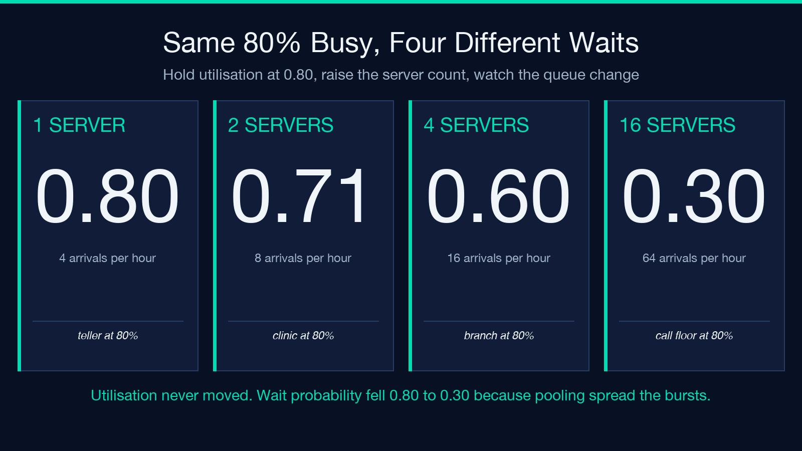
- c = 1, λ = 4/hour: wait probability 0.8000, expected line 3.2000, expected wait 0.8000 time units
- c = 2, λ = 8/hour: wait probability 0.7111, expected line 2.8444, expected wait 0.3556
- c = 4, λ = 16/hour: wait probability 0.5964, expected line 2.3857, expected wait 0.1491
- c = 8, λ = 32/hour: wait probability 0.4576, expected line 1.8306, expected wait 0.0572
- c = 16, λ = 64/hour: wait probability 0.3049, expected line 1.2195, expected wait 0.0191
Read the middle column twice. The expected number of people in line falls as you add servers, even as sixteen times more traffic flows through the system. The queue is shorter in absolute terms while serving sixteen times the arrivals per hour.
The mechanism is not mysterious, and it shows up in one comparison. With one server, each burst of two arrivals forces one of them to wait for a full service time. With sixteen, a burst of two finds fourteen idle servers and nobody notices. Pooling spreads the randomness across more capacity, which cuts the wait probability even though the average busy fraction never moved.
Erlang-C in one pass, plus a check that catches slips
The idle probability comes first, because the wait probability is built on top of it:
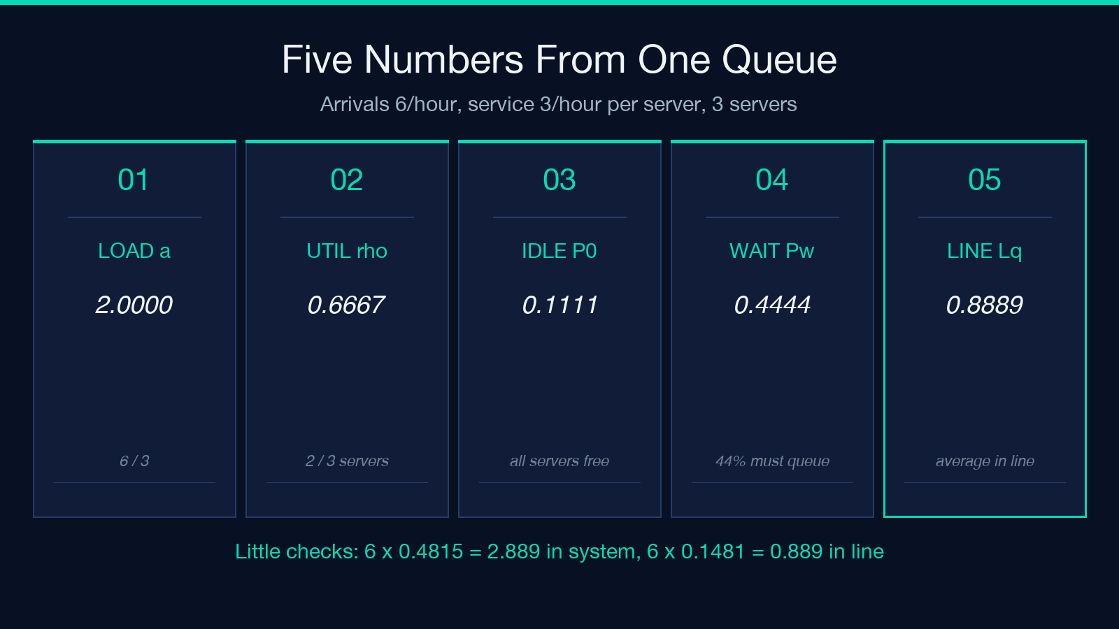
P0 = 1 / [ sum(n=0..c-1) a^n / n! + a^c / (c! (1 - rho)) ]
Then the Erlang-C probability that an arrival has to wait is Pw = P0 * a^c / (c! (1 - rho)), and the queue follows from it: Lq = Pw * rho / (1 - rho), L = Lq + a, W = L / lambda, Wq = Lq / lambda.
Take the classic bank, for example: λ = 6/hour, μ = 3/hour, c = 3. Offered load a = 2, utilization ρ = 0.6667, idle probability P0 = 0.1111. Erlang-C gives Pw = 0.4444 — fewer than half of all arrivals ever queue. The line averages Lq = 0.8889 customers inside a system holding L = 2.8889, so each customer spends W = 0.4815 time units in the branch, of which Wq = 0.1481 is plain waiting.
Now the check that catches almost any arithmetic mistake: Little’s law, L = λ·W and Lq = λ·Wq. The same calculator reports both products alongside the queue lengths, so the comparison is a glance, not a second worksheet. Here 6 × 0.4815 = 2.889 and 6 × 0.1481 = 0.889, which reproduces the two queue-length figures from the times. If those two products drift from Lq and L, the error is in P0 — usually a dropped term in the summation, which is the one place the formula is easy to get wrong by hand.
One extra server changes the shape, not the trend
The abstract comparison matters less than the decision in front of you. A clinic with arrival rate λ = 8/hour and μ = 5/hour per practitioner runs two servers. That gives ρ = 0.8000, Pw = 0.7111, Lq = 2.8444, and Wq = 0.3556 time units.
Add one practitioner. Utilization drops to 0.5333, and the same traffic now waits far less: the wait probability reduces to 0.2738, the line to 0.3129, and the expected wait to 0.0391 — a 9.09-fold cut. Add a second and Wq falls again to 0.0076, though the ratio between the third and fourth server is only about 5 to 1, and the absolute gap is now measured in minutes nobody will notice.
That asymmetry is the practical lesson. The first server you add to a congested system cuts an enormous amount of waiting time. The fourth cuts almost none, because almost none was left to cut. Staffing reviews that argue about utilization percentages are arguing about the least informative end of this curve; the useful argument is over which server count gets Wq below the wait your customers will tolerate.
Where the curve turns vertical
Fix c = 4 and μ = 5, then sweep the arrival rate. Each step below is the same system, one notch busier:
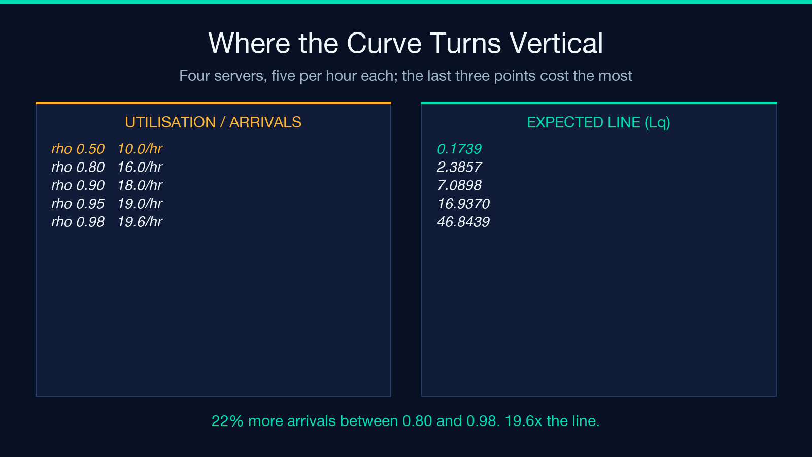
- ρ = 0.50, λ = 10/hour: Lq = 0.1739, Wq = 0.0174
- ρ = 0.70, λ = 14/hour: Lq = 1.0002, Wq = 0.0714
- ρ = 0.80, λ = 16/hour: Lq = 2.3857, Wq = 0.1491
- ρ = 0.90, λ = 18/hour: Lq = 7.0898, Wq = 0.3939
- ρ = 0.95, λ = 19/hour: Lq = 16.9370, Wq = 0.8914
- ρ = 0.98, λ = 19.6/hour: Lq = 46.8439, Wq = 2.3900
From 0.50 to 0.80 — a thirty-point move — the observed line grows by a factor of 13.7. From 0.80 to 0.90, ten points, it triples. From 0.95 to 0.98, three points of utilization, the expected line nearly triples again. The last three points cost more than the first thirty.
This is the honest reason utilization targets break down: 85% and 90% sound like neighbouring policies and behave like different businesses, and the data above is the whole argument. The same 5-point increase is nearly free at one end of the curve and ruinous at the other, and the curve’s shape depends on c, so a target imported from a team with a different server count is not a target at all.
The inputs it refuses, and why refusal is correct
Feed the bank above through c = 2 instead of c = 3 and the answer is not a large number — it is a rejection. With λ = 6 and μ = 3, two servers give ρ = 1.0 exactly, and the request is refused as unstable: offered load 2.0 against 2 servers, with the note that the line would grow without bound.
That refusal, reported as an error and not as a number, is the most useful thing the tool does. Each formula in this article is a steady-state result, and a steady state exists only while ρ is strictly below 1. At ρ ≥ 1 arrivals outpace service, the queue grows linearly with time forever, and the steady state breaks: there is no average to report. A calculator that printed a finite wait for an overloaded system would be lying politely; this one declines.
The bounds are worth knowing before you type: c must be an integer from 1 to 20, decimal places from 0 to 8, and both rates positive. Paste a peak-hour pair into the M/M/c calculator and the rejection arrives before you can argue with it. There is also a second guard behind the first — if ρ is so close to 1 that any metric becomes non-finite, the run is rejected as numerically unstable and asks for rates that are farther apart. At ρ = 0.99999 the 1 - rho denominators are absorbing float error faster than the formula can carry it, and the honest output is no output.
What the model never saw
The M/M/c queue is a model, and its two Ms are load-bearing assumptions, not decoration.
The first M is Poisson arrivals, which means the time between arrivals is exponentially distributed and its coefficient of variation is exactly 1. Real traffic — support tickets after an outage, patients on a Monday morning, orders during a flash sale — arrives in clumps, with a coefficient far above 1; the case of an outage is the extreme, where all the waiting figures here collapse at once. Burstier arrivals than Poisson reduce all the waiting figures here to optimism.
The second M is exponential service times, again coefficient of variation 1. Real service is usually more consistent than that, and lower service variability shortens queues; on that axis the model errs conservatively. The two errors push in opposite directions, which is convenient for the model and inconvenient for anyone who wants to know which one dominates. I did not have a real arrival trace to test against, so I cannot tell you the net direction for your workload — only that both effects are there.
Three more assumptions sit underneath. Customers wait in one shared first-come-first-served line, which is the pooling assumption that produced the 71% versus 30% gap; give each server its own private queue and the benefit largely evaporates. No one abandons, so Wq is the wait of someone who stays. And servers are identical — no trainee on one desk, no specialist on another. A week of real arrival data will tell you how far your case drifts from all three; the formula cannot.
What to put on the staffing review
Three numbers belong in the review, and utilization is not one of them.
Put the wait probability first, because it answers the question a customer experiences: what fraction of arrivals end up queueing at all. Put the expected wait Wq next, in the same time units your service level is written in. Put the server count that holds Wq under target third, and treat utilization as an output you report afterwards, not a dial you aim.
Then repeat it for each peak hour, not for the day. A system averaging 60% utilization across a week can sit at 0.95 for two hours each Monday, and the average will describe neither state. Run the arithmetic for each peak, not for the aggregate. When a single server is the honest model, the M/M/1 variant is the shorter path, and the category page for math and number tools holds both.
Explore more tools at elysiatools.com.
I came into this expecting utilization to be the safe, conservative number — the one you quote when you want to leave room. It is not a number you can quote alone. Eighty percent is 0.80 of a teller’s day, 0.71 probability of waiting at two servers, and 0.30 at sixteen, and the formula that separates those outcomes takes three inputs, not one. So when a staffing review opens with utilization, is the honest question whether the number is high — or which server count produced it?
本文有中文版:80% 的利用率,是两个不同的队列
