# 8 Free Chemistry Visualizations That Make Abstract Concepts Click
In 2019, a colleague of mine spent three hours trying to understand why phenolphthalein turns pink at pH 9.3 but not at pH 8. She had the Henderson-Hasselbalch equation memorized. She could write it down correctly. She could solve for pH given a ratio. What she couldn’t do was picture why the ratio of ionized to unionized indicator molecules shifted so sharply at that particular pH.
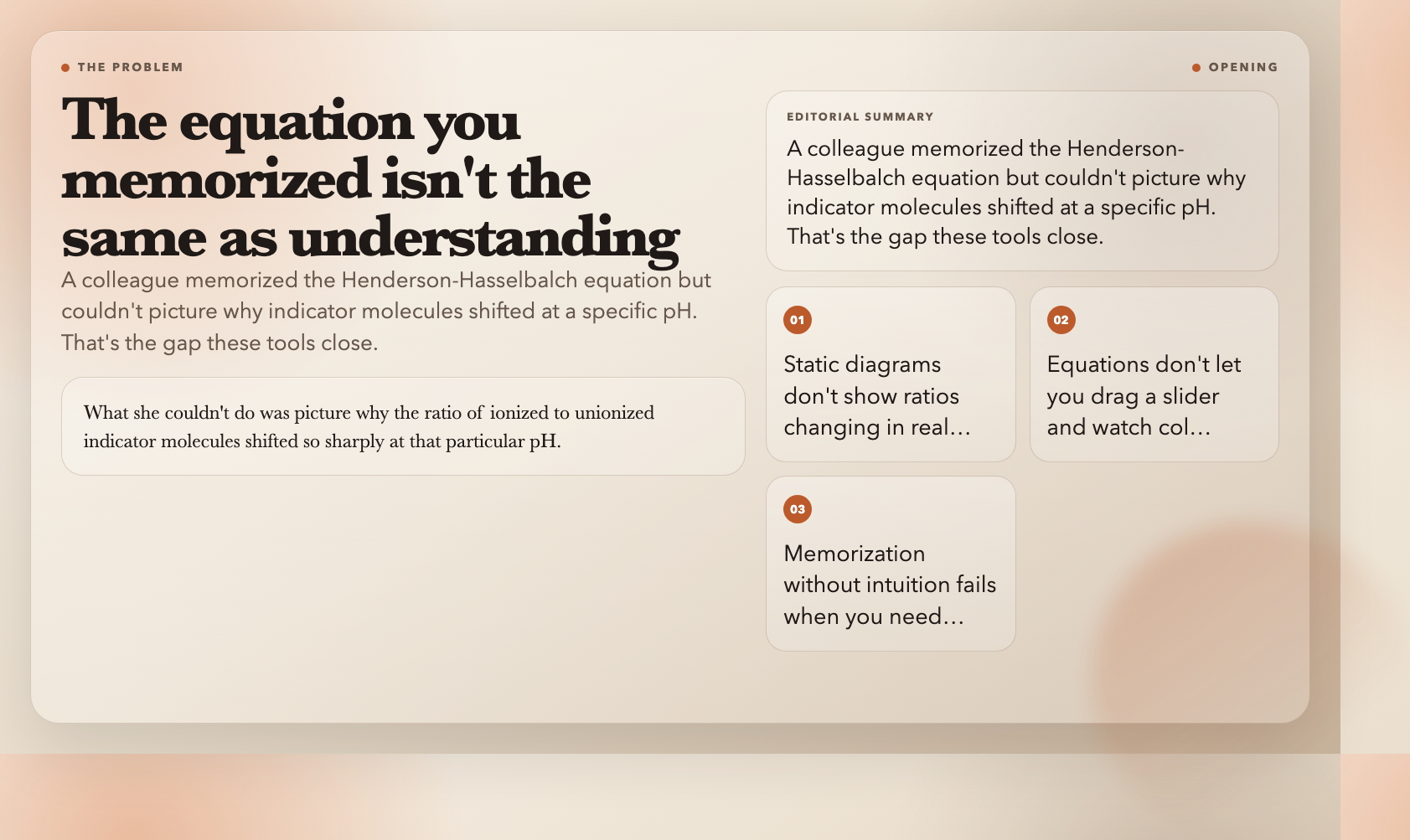
Static diagrams don’t show you ratios changing in real time. Equations don’t let you drag a slider and watch colors transition.
Here are eight free interactive visualizations that close that gap.
—
1. Acid-Base Indicators
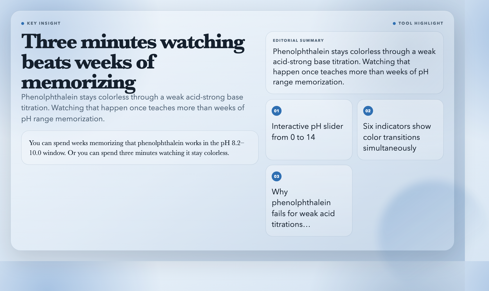
Drag a pH slider from 0 to 14 and watch six common indicators — phenolphthalein, methyl orange, litmus, bromothymol blue, methyl red, thymol blue — change color simultaneously. Each one has its documented transition range displayed on a real gradient, so you see exactly why phenolphthalein is useless for titrating weak acids against strong bases (equivalence point falls outside its range).
This is the visualization I wish I’d had during my undergraduate analytical chemistry lab. You can spend weeks memorizing that phenolphthalein works in the pH 8.2–10.0 window. Or you can spend three minutes watching it stay colorless through a weak acid titration, and never forget why.
Try Acid-Base Indicators free →
—
2. Arrhenius Equation
Two views: a standard k-vs-T plot showing exponential growth in reaction rate constant as temperature rises, and an Arrhenius plot (ln k vs 1/T) where activation energy becomes a literal line slope. Adjust Ea and the pre-exponential factor A, and both plots respond in real time.
Here’s the number I keep coming back to: according to the van ‘t Hoff rule, raising temperature by 10°C roughly doubles reaction rate for many reactions. For a high-activation-energy decomposition reaction, the same 10°C jump might produce a 4x or 5x increase. You can read that fact in a textbook, or you can see it in the curvature of the k-T plot. The difference in understanding is substantial.
Try the Arrhenius Equation visualization free →
—
3. Chromatography Principles
Chromatography separates mixtures by making compounds travel at different speeds through a column. This tool animates the process — you watch peaks emerge on a chromatogram in real time, adjust capacity factors to change retention times, and see how resolution (R) between adjacent peaks responds to column length, flow rate, and peak width.
The resolution formula R = 2(tR2 – tR1)/(w1 + w2) is manageable once you have an intuition for what each variable does. Adjust the peak width slider from narrow to wide and watch R collapse. Then shorten the column and watch it happen again. The formula stops being abstract.
Try Chromatography Principles free →
—
4. Buffer Solution
Buffers are everywhere — blood plasma, cellular fluid, preserved foods — and they work by resisting pH change. This visualization shows you exactly why. Add acid or base to a buffered solution and watch the pH barely move. Then do the same to unbuffered water and watch it plummet or spike.
The most striking moment in the visualization is the titration curve comparison: the buffered solution shows a long, flat plateau where pH barely changes even as you add substantial acid or base. The flatness of that plateau is the buffer’s capacity — and seeing it makes the entire concept obvious in a way no equation can.
Try Buffer Solution visualization free →
—
5. Enzyme Kinetics
Michaelis-Menten kinetics visualized as a real hyperbolic curve: reaction velocity on one axis, substrate concentration on the other. You adjust Km and Vmax and the entire curve shifts. A Lineweaver-Burk linearization plot updates simultaneously — which matters because competitive, non-competitive, and uncompetitive inhibition each produce a distinct signature on that linear plot.
Pharmaceutical researchers use these plots constantly. The cancer drug imatinib, for instance, works as a competitive inhibitor of the BCR-ABL tyrosine kinase — and you can see exactly what that looks like on a Lineweaver-Burk chart. This tool won’t teach you drug design, but it will give you the visual foundation that makes the drug design literature readable.
—
6. Weak Acid Ionization
For a weak acid in water, the fraction that ionizes depends on both concentration and Ka. This visualization shows the equilibrium [HA] ⇌ [H⁺] + [A⁻] as a dynamic system: drag a slider to change initial concentration or Ka, and watch the ratio of ionized to unionized forms shift in real time.
This matters more than it sounds. The degree of ionization determines whether a drug can cross the blood-brain barrier (only the unionized form crosses efficiently). It determines how effective a preservative is. It determines what happens in your mitochondria during intense exercise when lactic acid builds up. Getting the intuition for why weak acids behave differently from strong acids starts here.
Try Weak Acid Ionization free →
—
7. Le Chatelier’s Principle
Perturb a system at equilibrium — add reactant, remove product, change temperature, adjust pressure — and watch the system shift to compensate. The tool makes it immediate: stress a reaction, see concentrations redistribute, watch the equilibrium constant either hold steady or (when temperature changes) recalculate.
Students routinely confuse concentration perturbations with temperature perturbations because the math looks similar. This visualization separates them visually. When you add reactant and watch the forward reaction rate spike, then settle back — that’s a different dynamic from raising temperature and watching every rate change because the equilibrium constant itself changed. Seeing the two cases side by side eliminates the confusion permanently.
Try Le Chatelier’s Principle free →
—
8. Battery Principles
Electrochemical cells explained through oxidation-reduction reactions: galvanic cells (batteries that produce electricity), electrolytic cells (batteries that consume electricity), standard electrode potentials combining into cell potentials. You can trace electron flow through the external circuit, watch ions move through the salt bridge, and see why the lithium-ion chemistry in your phone works differently from the lead-acid chemistry in a car battery.
The practical implication is hard to ignore: battery degradation in lithium-ion cells comes from solid-electrolyte interphase (SEI) layer growth on the anode — a side reaction that consumes lithium ions. Once you can see the electrochemical potential landscape where this side reaction competes with the main charge-storage reaction, the “why batteries age” question stops being mysterious.
—
The Gap That Remains
These eight tools cover equilibria, kinetics, and electrochemistry with genuine interactivity. What they don’t cover — what almost no free tool covers — is computational chemistry visualization.
The quantum mechanical level: molecular orbital shapes, electron density surfaces, transition state geometries, Hartree-Fock optimization trajectories. The best free tools for these are PyMOL, Avogadro, and Gabedit, all of which require installation and significant learning curves. There is no browser-based, no-install, interactive visualization of a molecular orbital that a high school student can use without 45 minutes of setup.

That gap matters because computational chemistry is becoming central to drug discovery, materials science, and catalyst design. The tools above will give you a solid grounding in classical chemistry. Closing the gap to the quantum level requires building the browser-based computational visualization layer that doesn’t yet exist — which is as good a problem statement as any for someone looking to build something useful.