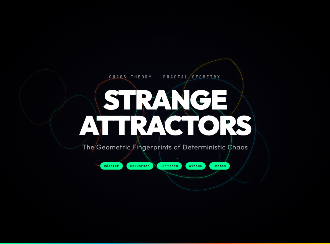
Strange Attractors: Where Chaos Draws Its Own Shape
Pick any point in 3D space near a strange attractor and trace where the system goes next. Do it again. Keep going. Eventually — after thousands of iterations — the shape that emerges isn’t a line, isn’t a circle, isn’t a surface. It’s something stranger: a fractal object with infinite detail, where every small patch resembles the whole, and where two trajectories that start inches apart will diverge exponentially but never escape the same ghostly volume of space.
Strange attractors are the geometric fingerprints of chaos. They appear in weather models, electronic circuits, fluid turbulence, and chemical reactions. And they’re one of the most visually stunning objects in all of mathematics.
What Makes an Attractor Strange

In ordinary dynamics — say, a pendulum with friction — a system’s long-term behavior settles into something simple: a point, a circle, a torus. These are “attractors” because nearby trajectories are drawn toward them. They’re not strange.
Strange attractors are different. They arise in nonlinear systems where small differences amplify exponentially. The hallmark is the fractal dimension — the structure has detail at every scale, and zooming in never reveals a smooth surface. Instead, you find more of the same intricate geometry, endlessly.
The Lorenz attractor (1963) was the first to be widely recognized. Edward Lorenz discovered it accidentally while running a simplified weather simulation. He noticed that his starting conditions — rounded from six decimal places to three — produced wildly different weather outcomes. The butterfly-shaped cloud of trajectories he mapped became the icon of chaos theory.
But Lorenz is just one example. The Rössler attractor has a characteristic folded ribbon structure. The Halvorsen attractor spirals outward in a distinctive radiating pattern. The Clifford attractor produces swirling, almost organic shapes. Each has its own personality, encoded in a handful of differential equations.
Seven Systems, One Interface

The Strange Attractors Gallery on ElysiaTools lets you explore seven distinct chaotic systems side by side through the same controls: Rössler, Halvorsen, Clifford, Aizawa, Thomas, Dadras-Momeni, and Sprott.
Each system is defined by a set of coupled differential equations. The Rössler attractor, for example, uses:
dx/dt = −y − z
dy/dt = x + ay dz/dt = b + z(x − c)
With parameters a = 0.2, b = 0.2, c = 5.7, the system traces its characteristic spiral. Change just one parameter and the geometry transforms — periodic windows appear, chaos disappears, the attractor folds differently.
What makes this gallery useful is that it exposes the parameters directly. Sliders let you vary each coefficient in real time. Watch how the Aizawa attractor — known for its toroidal structure — changes shape as you nudge its parameters. See the Dadras-Momeni system shift from periodic to chaotic behavior. The strange attractors tool gives you that control.
Why Fractal Dimension Matters
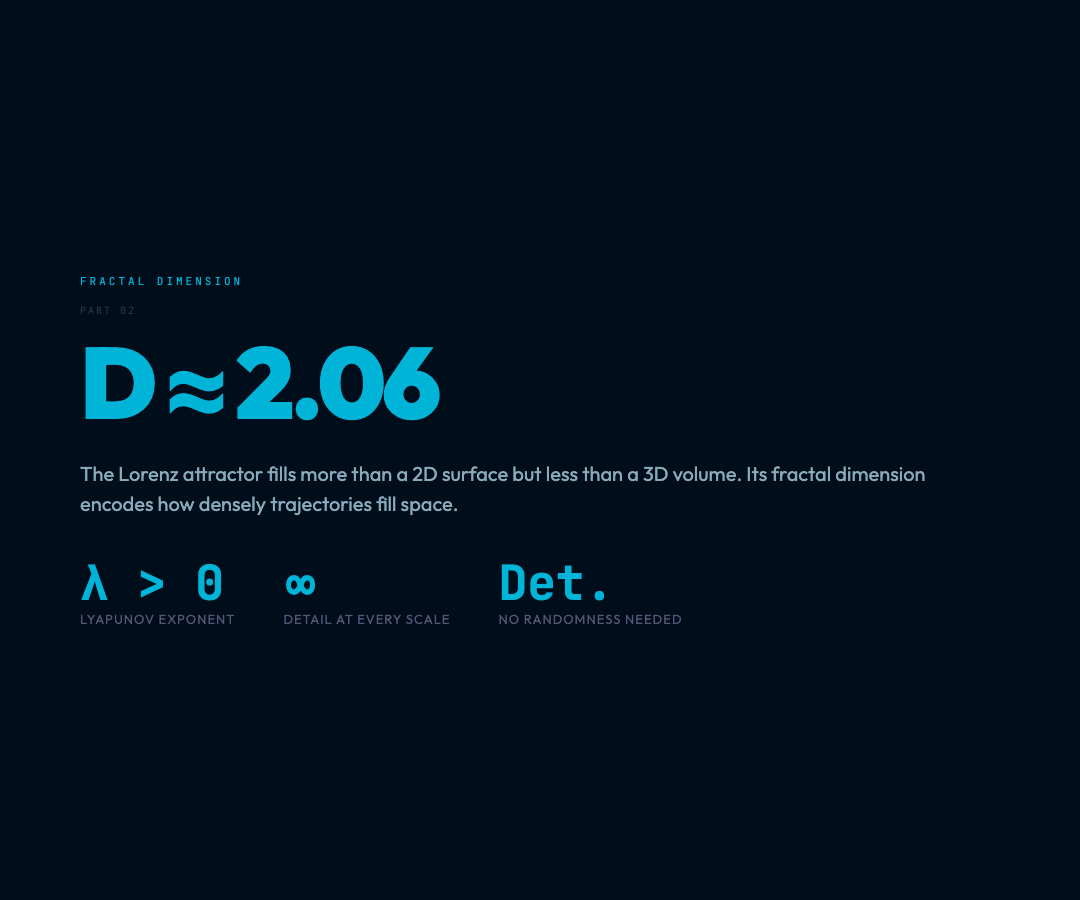
One of the deepest properties of strange attractors is their Lyapunov exponent — a number that measures how fast nearby trajectories diverge. A positive Lyapunov exponent is the mathematical definition of chaos: predictability gives way to exponential divergence, but the system remains confined to the attractor’s volume.
From this exponent you can compute the fractal (Hausdorff) dimension — which is almost never an integer. The Lorenz attractor has a dimension of approximately 2.06. The Rössler attractor sits around 2.1 to 2.4 depending on parameters. These aren’t holes in the geometry; they’re measures of how densely the trajectories fill space.
This fractional dimension is the “strange” in strange attractor — a shape so intricate that it occupies more than a surface but less than a volume. It’s a geometry that only makes sense in fractional terms.
Chaos Is Deterministic
The most counterintuitive feature of strange attractors is that they’re produced by deterministic equations — no randomness is involved. Give the same initial conditions to a chaotic system and you’ll get exactly the same trajectory, every time. The unpredictability doesn’t come from noisy inputs. It comes from extreme sensitivity to initial conditions.
This is why chaos is sometimes called deterministic chaos. The future is fully determined by the present, but you can never know the present precisely enough to predict the distant future. This has real-world consequences: weather forecasting, stock markets, brain activity, and planetary orbits all exhibit chaotic behavior that limits how far ahead prediction is possible.
Try It Yourself
The best way to understand strange attractors is to manipulate them directly. Change the rotation speed to watch how the 3D structure orients in space. Adjust the trail length to see how individual trajectories trace out the global shape. Toggle depth coloring to reveal where in the parameter space the trajectory spends the most time.
Spend a few minutes with the Strange Attractors Gallery and you’ll develop an intuition for how chaotic systems behave — that same mix of inevitability and surprise that makes chaos theory one of the most seductive branches of mathematics.