The Algorithm That Could Make Your Models Converge 10x Faster — If You Can Afford It
Every deep learning practitioner knows the ritual. You set your learning rate, watch the loss curveplummet, plateau, plateau some more, and then — finally — declare victory. Gradient descent has been the workhorse of machine learning for decades. But there’s another algorithm, sitting in textbooks and optimization courses, that can converge in a fraction of the iterations: Newton’s method.
The problem? It comes with a price tag most of us can’t afford to pay.
Two Algorithms, One Visualization
Open the Gradient Descent / Newton Method visualization on ElysiaTools and you see something immediately striking. Both algorithms start at the same point on the same loss surface. Gradient descent inches forward, methodically, step by step. Newton’s method leaps — not because it has a higher learning rate, but because it knows where the valley is. It doesn’t just follow the slope; it reads the curvature of the entire landscape.
This is the fundamental difference between first-order and second-order optimization.
Gradient descent uses only the first derivative — the slope — to decide where to step next. It’s like hiking down a mountain in thick fog: you feel the ground tilting downward and take a step that way. Simple, reliable, but blind to what’s over the next ridge.
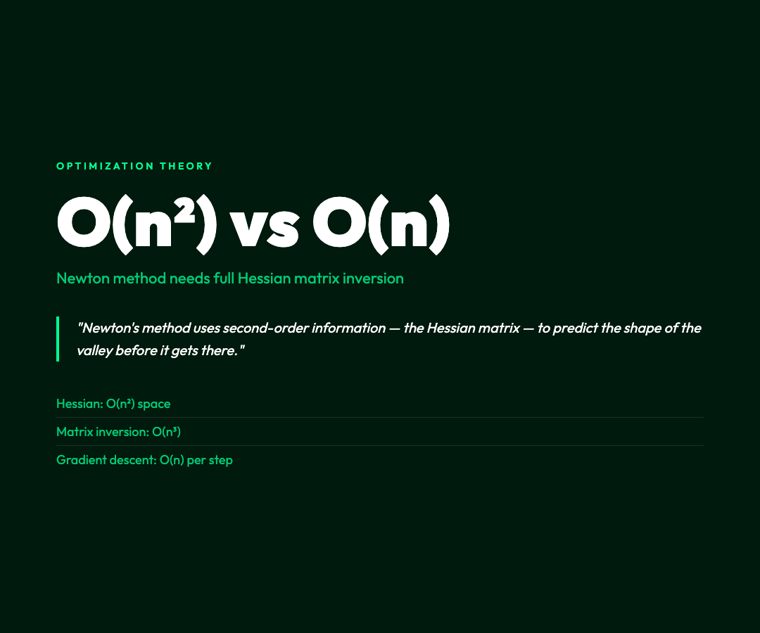
Newton’s method uses second-order information — the Hessian matrix of second derivatives — to predict the shape of the valley before it gets there. It’s like having a contour map in that fog. The steps are larger and more deliberate because the algorithm knows the full topology of the terrain.
Why Gradient Descent Won
If Newton’s method is theoretically superior, why does gradient descent dominate machine learning?
The answer is arithmetic. Newton’s method requires computing and inverting the Hessian matrix — a square matrix of second derivatives with one entry for every pair of parameters. A model with 1 million parameters has a Hessian with 1 trillion entries. Inverting that matrix is O(n³) in the best case. For modern large language models with hundreds of billions of parameters, this is computationally intractable.

Gradient descent, by contrast, scales linearly with the number of parameters. It’s memory-efficient, parallelizable, and has decades of engineering behind it. The momentum trick, adaptive learning rates (Adam, RMSprop), and learning rate schedules have made it robust enough to train on billions of examples.
This is why the machine learning field made a pragmatic trade: more iterations in exchange for cheaper-per-iteration computation. We sacrifice Newton-level efficiency for gradient descent-level feasibility.
Where Newton’s Method Still Wins
But “cheaper per iteration” doesn’t always mean “faster to convergence.” For small-to-medium problems — where the Hessian fits in memory — Newton’s method can be dramatically faster. In scientific computing, control theory, and certain engineering applications, practitioners still reach for it.
The visualization lets you test this yourself. Switch between four objective functions:
– Convex quadratic: A simple bowl. Both methods reach the minimum cleanly, but Newton’s method takes roughly 3-5 iterations versus gradient descent’s 50-100 depending on learning rate. – Rosenbrock: A banana-shaped valley. Gradient descent zigzags painfully along the long narrow valley. Newton method navigates it with far fewer steps. – Himmelblau: Multiple local minima. Both methods find one of the minima — which one depends on where you start. This is a useful reminder that optimization algorithms don’t guarantee global optima. – Rastrigin: A highly oscillatory surface with many local minima. Both algorithms struggle here, illustrating a fundamental limitation: no local optimization method can guarantee finding the global minimum in general.
The Practical Takeaway
If you’re training a neural network with 100 million parameters, gradient descent — with all its engineering sophistication — is the only viable choice. The math simply doesn’t work for Newton’s method at that scale.
But if you’re optimizing a logistics model with a few thousand parameters, or solving a control engineering problem where you need fast convergence, consider reaching for a second-order method. Quasi-Newton algorithms like L-BFGS offer a middle ground — they approximate the Hessian implicitly, avoiding the full matrix storage cost while still benefiting from curvature information.
The visualization at ElysiaTools is a clean way to build intuition for this trade-off. Watch the two trajectories diverge — literally — and you’ll understand viscerally why the machine learning field settled on gradient descent, and where second-order methods still earn their keep.

The valley is out there. Gradient descent just walks there one step at a time. Newton’s method flies — when it can afford the fuel.
Try it: Gradient Descent / Newton Method — adjust learning rates, switch objective functions, and click anywhere on the contour plot to set your own starting point.