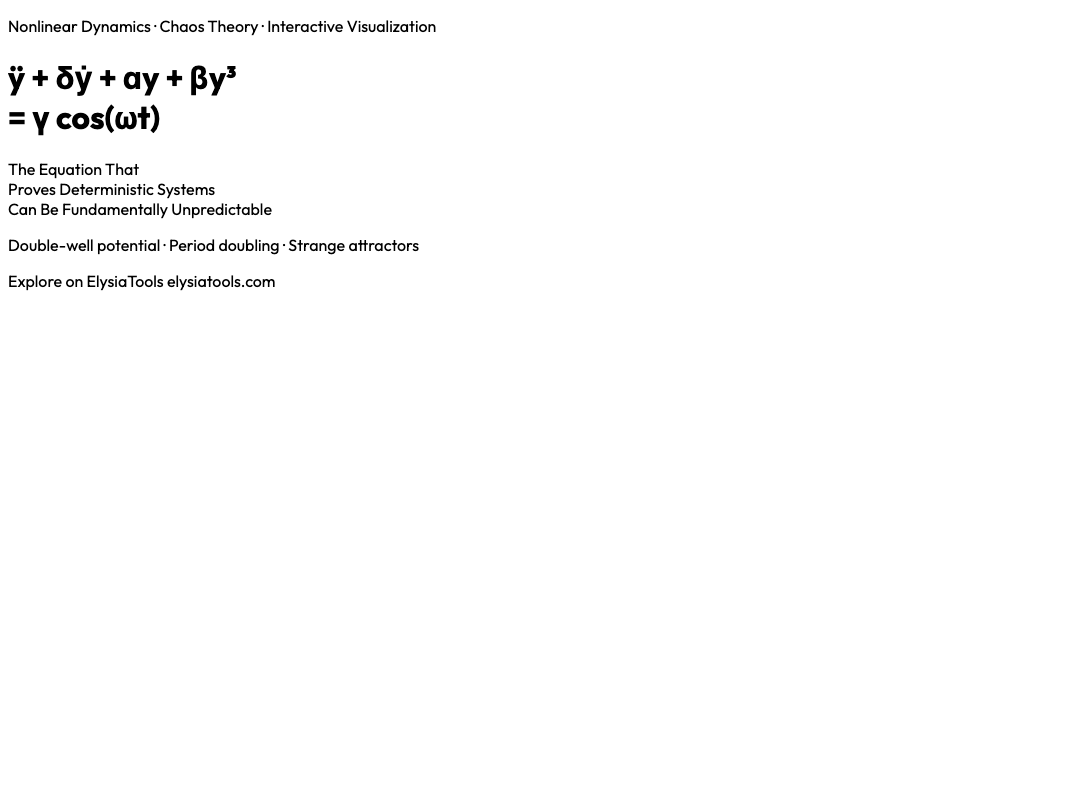
The Simple Oscillator That Proves Deterministic Physics Can Be Fundamentally Unpredictable
In 1918, a young engineer named Georg Duffing wrote down an equation that would haunt dynamical systems theory for the next century. It looked innocent enough — just a slightly modified version of the ordinary harmonic oscillator that every physics student learns. But beneath its deceptively simple form lay something profound: a single deterministic equation capable of producing behavior so unpredictable that no amount of computational power could save you from it.
The equation is:
ÿ + δẏ + αy + βy³ = γ cos(ωt)
Add a tiny bit of damping (δ), a cubic nonlinearity (βy³), and a periodic driving force (γ cos(ωt)) to an ordinary spring, and you get a system that can do something extraordinary — it can become chaotic. Not randomly chaotic, mind you. Perfectly deterministic chaos, where the same equation produces trajectories that are unique, unrepeating, and utterly sensitive to the smallest changes in where you start.
This is the Duffing oscillator — and it’s one of the most important examples in all of nonlinear dynamics.
The Double-Well Potential: When a System Has Two Places to Rest
The magic of the Duffing oscillator lives in its potential energy function. Unlike a ordinary spring — where the restoring force is proportional to displacement (F = -kx) and there’s only one equilibrium point at y = 0 — the Duffing oscillator’s cubic nonlinearity creates a different landscape entirely.
When α < 0 and β > 0, the potential energy becomes:
V(y) = -½αy² + ¼βy⁴
This is the double-well potential: a two-humped landscape with two stable equilibrium points, one on each side of the origin. A particle in this system doesn’t just oscillate around a single center. It can settle into either well, oscillating gently at the bottom like a ball in a bowl. But if you give it enough energy — enough drive amplitude γ — it can clamber up and over the barrier between wells, jumping from one side to the other.
This well-switching behavior is where things get interesting. At low drive amplitudes, the particle oscillates peacefully in one well. Increase the drive amplitude slightly, and something strange happens: the oscillation period suddenly doubles. Increase it again, and it doubles again. Increase it a third time, and you’re in chaos — aperiodic, unpredictable, sensitive to initial conditions.
This is period doubling — the same route to chaos discovered by Feigenbaum in the logistic map, playing out here in a continuous, physics-based system.
Period Doubling: The Road to Chaos Paved in Twice
The period-doubling cascade in the Duffing oscillator is remarkably clean to observe. Set α = -1, β = 1, δ = 0.25, ω = 1, and start with γ = 0.20. The particle oscillates with a simple, repeating waveform — one bump per drive cycle. Now increase γ to 0.27. The oscillation still looks periodic, but if you wait long enough, you’ll notice it doesn’t repeat after one cycle — it takes two. The system has doubled its period.
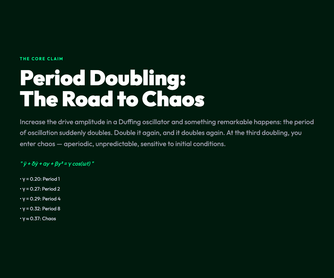
Increase to γ = 0.29, and it doubles again: four cycles per drive period. Push to γ = 0.32, and eight. At γ ≈ 0.37, the period becomes effectively infinite. There is no repeating pattern. The motion is chaotic.
What makes this cascade so elegant is that it happens in a continuous system governed by differential equations — not in a discrete map where you iterate a function. The same mathematics that describes population dynamics and electrical circuits is playing out in a mechanical system you can build in a lab.
Poincaré Sections: A Stroboscopic Window into Chaos
How do you tell whether a continuously oscillating system is periodic or chaotic? You use a Poincaré section — a technique named after the French mathematician Henri Poincaré, who essentially invented chaos theory decades before computers existed.
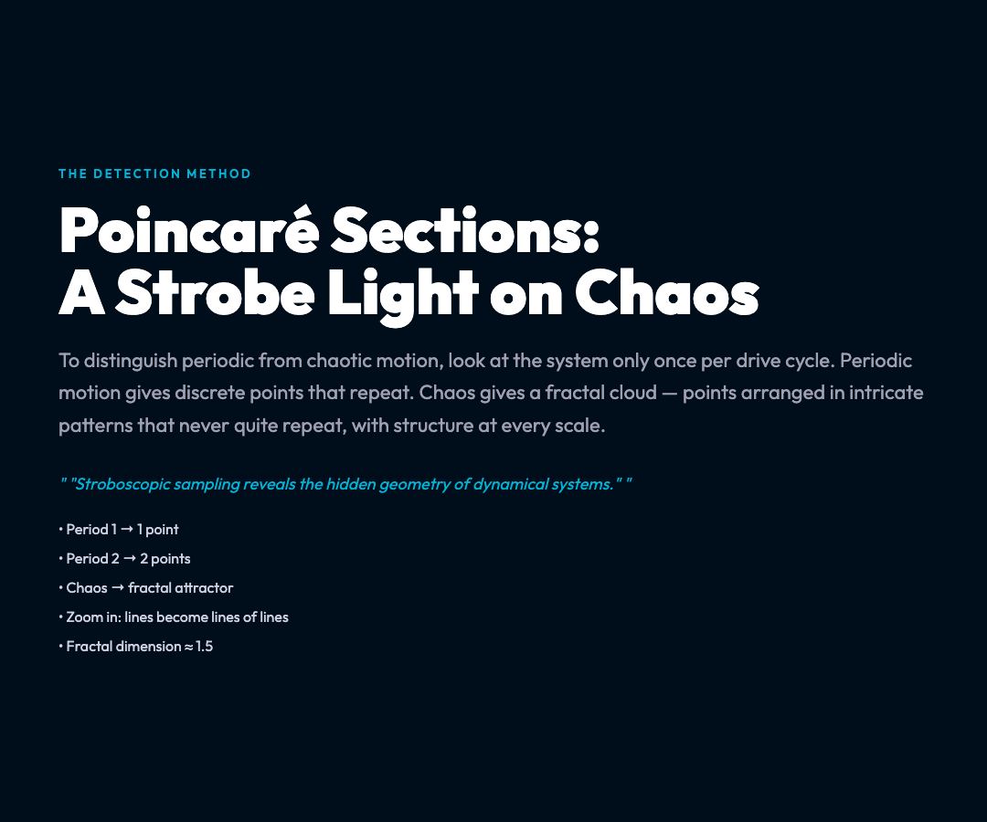
The idea is elegantly simple: instead of watching the continuous trajectory in phase space (velocity vs. position) at every instant, you only look at the system once per drive period. Stroboscopic sampling, in other words. You flash a light at the system at the same phase of every cycle and record where the particle is.
If the system is periodic with period 1, the Poincaré section shows a single point — the system returns to exactly the same state each flash. If the period has doubled to 2, you see two points. Period 4 gives four points. And if you’re in the chaotic regime, you don’t get points at all — you get a fractal cloud, a strange attractor with intricate structure that never quite repeats.
In the Duffing oscillator’s classic chaos configuration, the Poincaré section reveals a shape with clear fractal geometry. Points that look scattered reveal, on closer magnification, that they’re arranged in curved lines. Zoom in further, and those lines reveal themselves to be made of even finer lines. The structure has no characteristic scale — it looks similar at every magnification, a hallmark of fractal geometry.
The Double-Well Jump: When Chaos Means Escaping the Impossible
Perhaps the most dramatic manifestation of chaos in the Duffing oscillator is the phenomenon of well-switching — the chaotic jumping between the two potential wells. In the chaotic regime, the system doesn’t settle into either well permanently. Instead, it oscillates in one well for an unpredictable number of cycles, then suddenly escapes over the barrier and oscillates in the other well, then returns — or doesn’t.
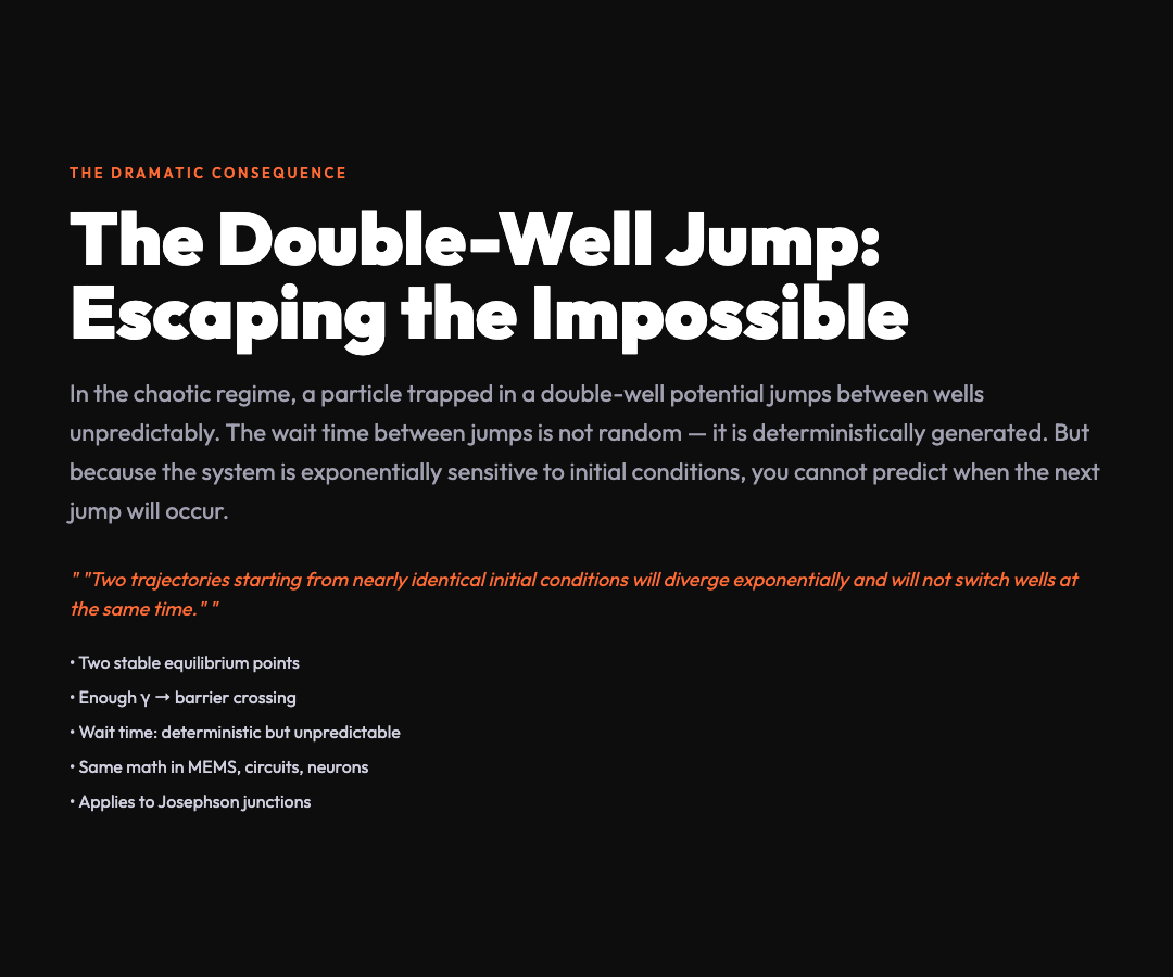
The wait time between jumps is not random in the stochastic sense. The underlying dynamics are completely deterministic. But because the system is exponentially sensitive to initial conditions, the wait time is effectively unpredictable in practice. Two trajectories starting from nearly identical initial conditions will diverge exponentially and will not switch wells at the same time.
This has profound implications for physical systems. A particle trapped in a double-well potential — a Josephson junction, a buckling beam, a nonlinear optical cavity — can exhibit spontaneous switching that looks random, even though it’s generated by deterministic chaos. Without knowing the exact initial conditions (which is impossible in any real experiment), you cannot predict when the next switch will occur.
Phase Space: Where Geometry Meets Physics
The phase portrait — a plot of velocity versus position — is where the geometry of chaos becomes visible. In a linear harmonic oscillator, the phase portrait is a perfect ellipse, closed and regular, repeating forever. In the Duffing oscillator, the phase portrait depends on the parameters.
For periodic motion, the phase trajectory is a closed loop — not an ellipse, but a distorted oval whose shape reflects the cubic nonlinearity. For period-doubled motion, the trajectory doesn’t close after one cycle, but after two — you see a figure-eight-like structure traced over two cycles. And in the chaotic regime, the trajectory never closes at all. It fills a region of phase space with intricate, non-repeating structure: a strange attractor.
The strange attractor of the Duffing oscillator is not a surface or a curve. It’s a fractal object — a set of points with fractional dimension, infinitely complex, that the trajectory approaches but never exactly repeats. Every path through phase space is unique. And yet all paths, for the same parameters, stay within the same attractor boundary. Chaos is not randomness — it’s hidden order of the most complicated kind.
Applications: From MEMS to Neurobiology
The Duffing oscillator is not merely a mathematical curiosity. It appears across physics and engineering wherever nonlinearities matter.
In microelectromechanical systems (MEMS), cantilever beams exhibit cubic restoring forces when deflected. When driven near resonance, these beams show the same period doubling and chaos as the Duffing equation. MEMS sensors designed for RF signal processing must account for these nonlinear effects — otherwise, the chaotic regime produces frequency instabilities that corrupt measurements.
In electrical circuits, a simple circuit with a diode exhibits Duffing-like nonlinear resonance. The van der Pol oscillator (a close cousin) describes the behavior of heart pacemaker cells and neural oscillations. The same mathematics that produces chaos in a driven circuit describes the irregular firing patterns in biological neurons.
In structural engineering, buckling beams under periodic loading follow equations similar to Duffing’s. An aircraft wing or a bridge under wind loading can exhibit chaotic vibrations if the driving frequency is in the wrong range — a fact that makes the Duffing oscillator essential reading for aerospace and civil engineers.
Try It Yourself
The Duffing oscillator is one of the most interactive and educational chaos visualizations available on ElysiaTools. You can adjust parameters in real time — damping δ, nonlinear coefficient β, drive amplitude γ, drive frequency ω — and watch the system transition between periodic and chaotic behavior instantly.
Try the “Classic Chaos” preset to see the period-doubling route. Switch to “Double Well” to watch the system jump between wells unpredictably. Enable the Poincaré section to see the fractal attractor emerge. The phase portrait, time-domain plot, and potential energy visualization all update simultaneously, giving you a complete picture of what’s happening.
It’s one of the clearest, most tactile introductions to deterministic chaos available — and it’s free.
Why This Matters
The Duffing oscillator teaches a profound lesson that extends far beyond physics: a system does not need randomness to be unpredictable. Deterministic equations, with no noise, no randomness, no quantum effects, can still produce behavior that is fundamentally impossible to forecast beyond a short time horizon.
This is the nature of chaos — not disorder, but hidden complexity that defeats prediction not because we’re ignorant, but because the mathematics itself makes long-term prediction impossible. The same principle applies to weather, to stock markets, to population dynamics, and to the human heart.
The next time someone says a system is “just deterministic” and therefore predictable, point them to the Duffing oscillator. An equation with three terms — a linear restoring force, a cubic nonlinearity, and a periodic drive — is all it takes to push a system beyond the edge of predictability, into a regime where the future is determined but unknowable.
ÿ + δẏ + αy + βy³ = γ cos(ωt)
Five symbols. Infinite complexity.