The Interactive Visualization That Shows Why Quantum Mechanics Freaks Everyone Out
An electron doesn’t go through one slit or the other — it goes through both. And until you look, it’s not even decided which path it took. That’s not a metaphor. That’s the math.
The quantum wave function collapse visualization on ElysiaTools lets you build superpositions of quantum states, watch them evolve in real time, and trigger measurements that shatter the superposition instantly. If you’ve ever wondered what “collapse” actually looks like mathematically, this is the tool that makes it viscerally real.
What a Wave Function Actually Is
Classical physics is straightforward: a particle has a position and a velocity, and those numbers determine everything. Quantum mechanics abandoned that premise in 1925, and physicists still argue about what replaced it.
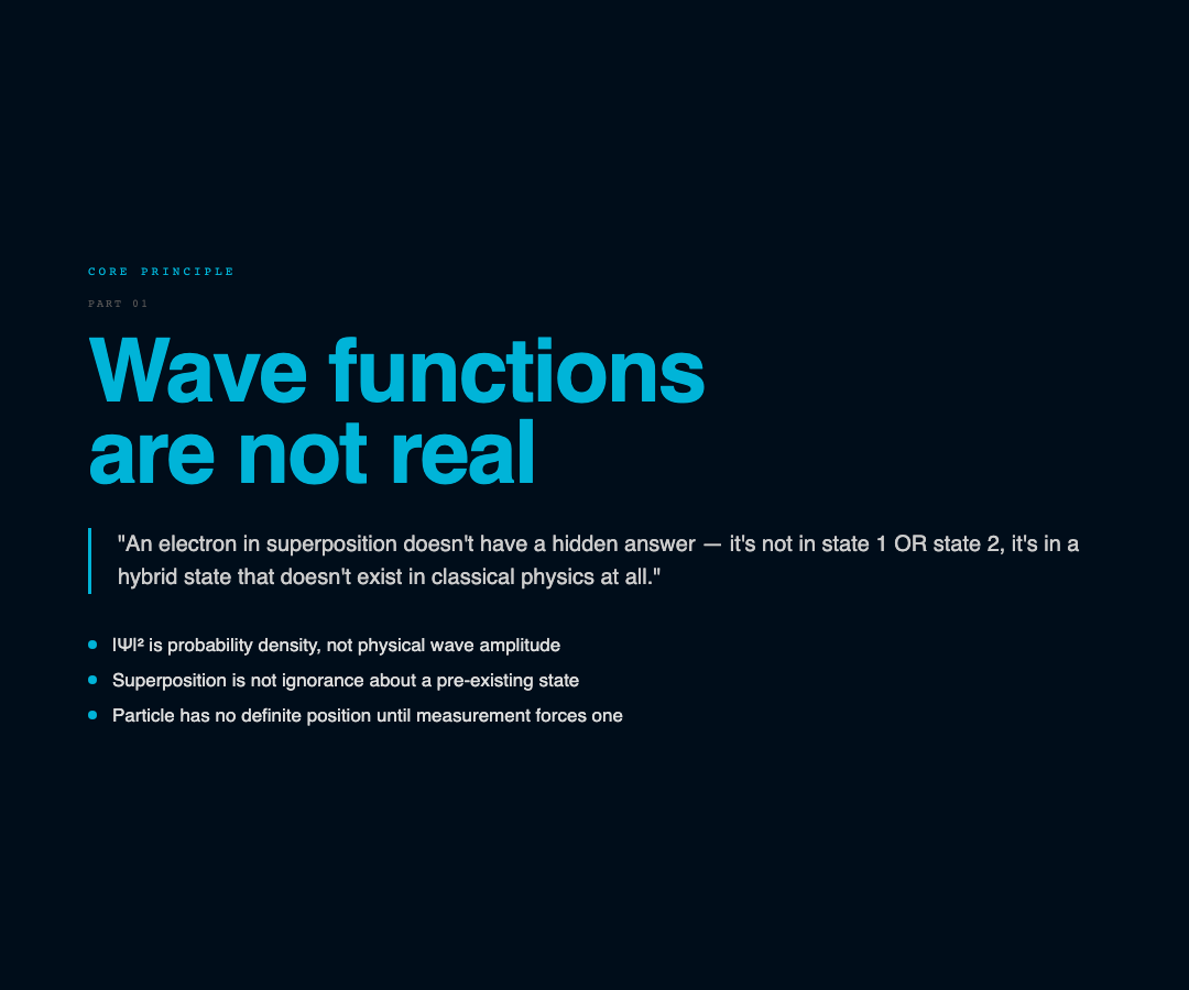
The wave function Ψ(x,t) is not a physical wave like sound or light. It’s a probability amplitude — a complex number whose absolute square |Ψ|² gives the probability density of finding the particle at position x if you measure it right now. Before measurement, the particle genuinely has no definite position. It’s spread out across space, interference-ready, until the moment you observe it.
This isn’t ignorance. It’s not that we don’t know the particle’s position — it’s that the particle literally doesn’t have one until measurement forces the issue.
Superposition: What It Actually Means
The visualization lets you superpose multiple energy eigenstates using adjustable coefficients cₙ. The system sits in a combined state:
Ψ(x,0) = c₁ψ₁ + c₂ψ₂ + c₃ψ₃ + …
Each ψₙ is a stationary state — an allowed energy configuration of the particle in the potential well. The coefficients are probabilities in disguise: |cₙ|² is the probability that measurement will find the system in eigenstate n.
Here’s the part that breaks intuition: the system isn’t secretly in one of these states while you look away. It’s genuinely in the superposition. Both states simultaneously. That phrase “both states simultaneously” gets repeated so often it starts to sound trivial. It isn’t. An electron in a superposition of “passed through slit 1” and “passed through slit 2” doesn’t have a hidden answer — it’s not in slit 1 OR slit 2, it’s in a hybrid state that doesn’t exist in classical physics at all.
Time Evolution: Where Interference Comes From
Each stationary state evolves in time with its own phase factor:
ψₙ(x,t) = ψₙ(x) · e^(-iEₙt/ℏ)
The key word is phase. Each component rotates at its own frequency, and because the energies Eₙ differ, the relative phases between components change continuously. When you plot |Ψ(x,t)|², you’re watching interference patterns form and dissolve as these phases drift in and out of sync.
Watch the double-well potential with two dominant states. The probability density doesn’t stay put — it sloshes from left to right and back, because the symmetric and antisymmetric combinations accumulate phase at different rates. This is quantum tunneling made visible in the probability landscape.
The Collapse: Measurement as Destruction
Press “Measure” in the visualization and watch what happens. The smooth, interference-rich probability distribution suddenly snaps into a single eigenstate. The system was in a superposition a fraction of a second ago, and now it’s in exactly one eigenstate. The other components don’t gradually fade — they vanish instantaneously across all of space.
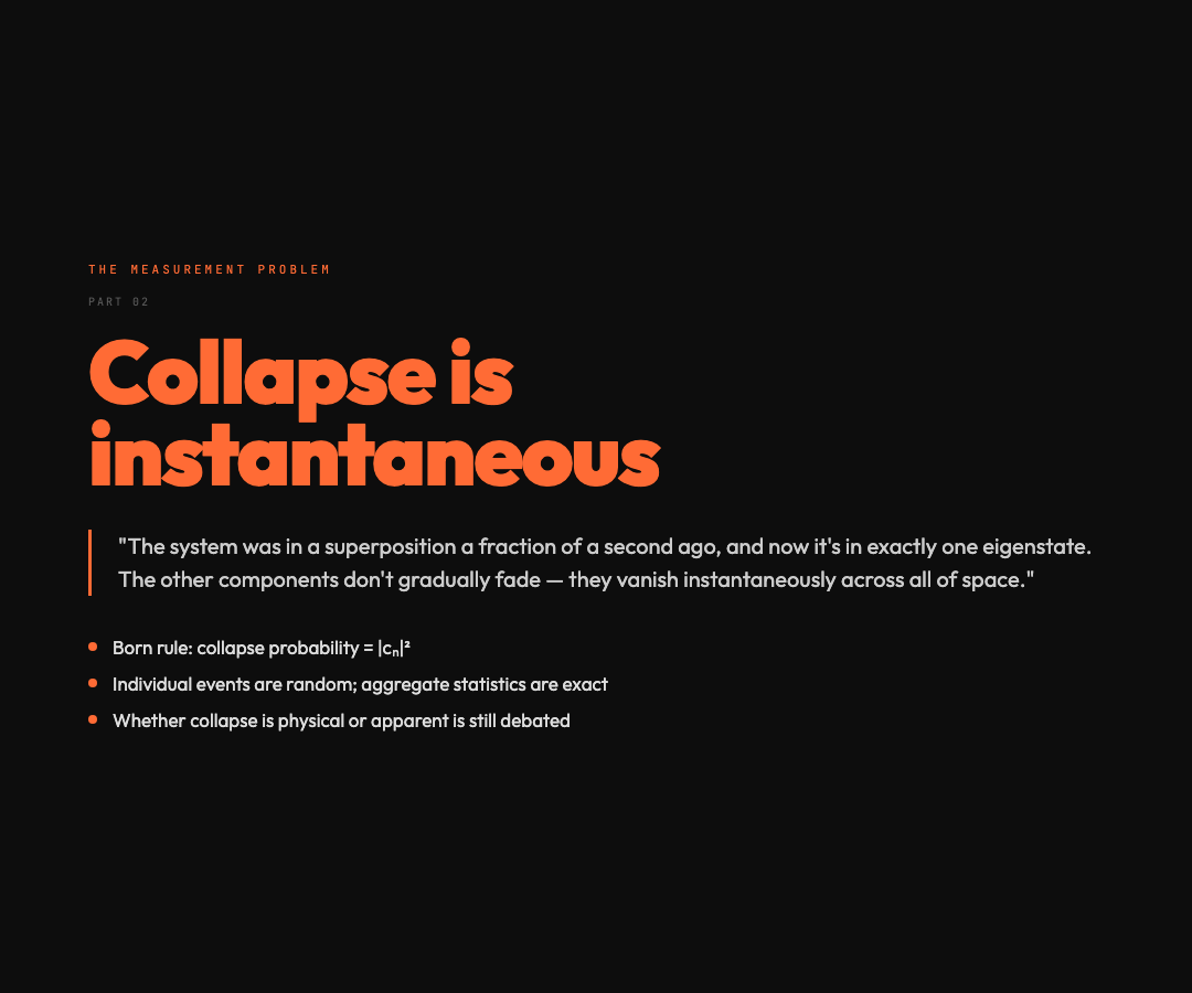
This is the Born rule in action (Max Born, 1926): the probability of collapsing to eigenstate n is |cₙ|². Run the same experiment 1000 times with identical coefficients, and you’ll get a distribution of outcomes matching those probabilities. The predictions are exact. Nobody disputes the numbers.
What physicists argue about is whether collapse is a real physical process or an artifact of how we describe the system. Copenhagen says collapse is physical — measurement triggers it. Many-Worlds says collapse never happens; instead, the universe branches and each outcome occurs in a separate branch. Decoherence says interaction with the environment (air molecules, thermal radiation, stray photons) suppresses interference so effectively that collapse becomes effectively irreversible without needing new physics.
All three make identical predictions for every experiment we can run. The debate is not about physics — it’s about what the math means.
Four Potential Wells, Four Quantum Lessons
Infinite Square Well: The simplest box. Energy levels follow Eₙ ∝ n², so spacing grows as n increases. The ground state has nonzero energy — zero-point energy — because you cannot simultaneously confine a particle to a small region and give it zero momentum. Heisenberg’s uncertainty principle is not a statement about measurement limits; it’s a structural feature of the math.

Finite Square Well: The walls are no longer impenetrable. Wave functions bleed into the classically forbidden region, decaying exponentially. This is quantum tunneling — a particle can briefly borrow enough energy to exist inside a barrier, as long as it gives it back quickly enough. The finite well supports only finitely many bound states, unlike the infinite well’s infinite ladder.
Harmonic Oscillator: V(x) = ½mω²x². Energy levels are equally spaced: Eₙ = (n+½)ℏω. This equal spacing means superpositions in the harmonic oscillator produce probability densities that oscillate with a perfectly fixed period — no revivals, no chaos, just clean periodic motion. This potential appears everywhere because any smooth minimum is locally harmonic. Molecular vibrations, phonons in solids, quantum fields — all built on this same structure.
Double Well: Two finite wells separated by a barrier. A particle starting in the left well will, through tunneling, spontaneously appear in the right well, then tunnel back. The oscillation frequency is set by the energy splitting between symmetric and antisymmetric states. This is not a classical particle bouncing back and forth — it’s a quantum particle simultaneously occupying both wells, with the tunneling rate determined by the barrier height and width.
What This Tool Actually Does For You
The tool isn’t a simulation of quantum mechanics — it computes and renders actual wave functions. You control the potential type, the number of energy levels, the superposition coefficients, and the animation speed. The Measure button performs an actual collapse according to the Born rule, with probability weights matching your coefficients.
The visualization renders the probability density |Ψ(x,t)|² in real time as interference patterns form and dissolve. The energy spectrum panel shows your |cₙ|² weights visually. The collapse animation shows you exactly what gets destroyed when measurement occurs.
For students encountering quantum mechanics for the first time, this tool bridges the gap between the equations and physical intuition. For those who’ve studied QM before, watching a superposition evolve and then watching it collapse gives a visceral feel for what those abstract amplitudes actually do.
Try It Yourself
The Quantum Wave Function Collapse visualization runs entirely in the browser. Start with the infinite square well, set two dominant coefficients (say 0.7 and 0.3), and watch the probability density oscillate. Then press Measure and watch it snap. Run it again. And again. The Born rule is statistical — individual outcomes are random, but the pattern over many runs is deterministic.
That’s quantum mechanics in one sentence: individual events are random, aggregate statistics are exact. Whether that randomness is fundamental or reflects something deeper we haven’t figured out yet — that question is still open.
This visualization is part of the ElysiaTools physics collection — interactive simulations that make invisible mathematics physically tangible.