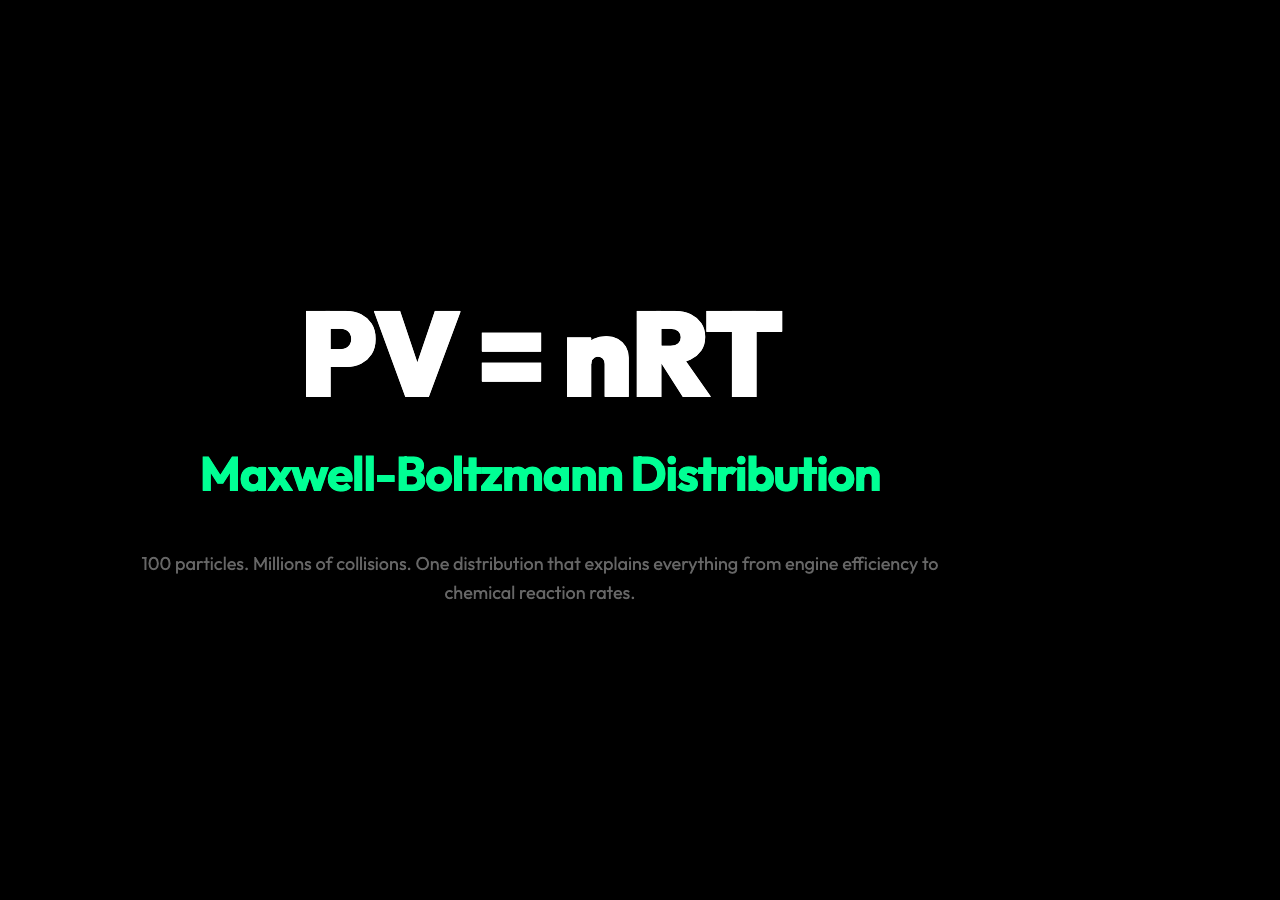
Why 100 Tiny Particles Teaching Us More About Temperature Than Any Textbook
The moment you watch molecules ricochet off container walls at 500 meters per second — and call that pressure — is the moment statistical mechanics stops being abstract and becomes visceral. That’s what makes the ideal gas simulation so quietly effective: it doesn’t just show you the Maxwell-Boltzmann distribution. It makes you feel why temperature is not a thing, but a story averaged across millions of collisions.
The Setup: One Container, 100 Particles, One Equation
At its core, the simulation models what every introductory thermodynamics course introduces in week three: an ideal gas. Unlike real gases — which have intermolecular forces, volume exclusion, and quantum effects at high density — an ideal gas assumes particles that interact only through elastic collisions. No attraction, no repulsion, just billiard-ball dynamics at every instant.

The physical constants embedded in the code reveal how carefully the simulation is constructed. Boltzmann’s constant kB = 1.380649×10⁻²³ J/K sits at the heart of every calculation. The default temperature is 300 K (room temperature, roughly 27°C). Particle mass is set to 28.0 atomic mass units — approximately nitrogen gas (N₂), the dominant component of air. Each molecule carries kinetic energy that scales linearly with temperature:
Eₖ = (3/2)kBT
At 300 K, a nitrogen molecule travels at roughly 517 m/s. The simulation initializes 100 such particles with random initial velocities and lets the physics run. The canvas shows them in continuous motion — colliding with each other, bouncing off walls — and the distribution panel plots their speed distribution in real time.
What makes this visually compelling is the gap between intuition and reality. Most people imagine molecules moving at roughly the same speed. The Maxwell-Boltzmann distribution says otherwise: at any given temperature, a wide range of speeds exists, with a long high-speed tail. The simulation’s color-coding — faster particles in warm colors, slower in cool — makes this distribution tangible rather than algebraic.
What the Distribution Actually Shows
The Maxwell-Boltzmann distribution isn’t just a curve on a graph. It’s a consequence of asking: given N particles with total energy E, how many ways can that energy be distributed? The distribution that maximizes entropy — the most probable macrostate — turns out to be the Maxwell-Boltzmann curve.

In the simulation, the distribution panel updates every few frames. Watch long enough and you’ll notice the curve settling into a stable shape. Change the temperature slider and the entire distribution shifts — the peak moves right (faster average speed), the curve widens (greater variance), and the tail extends further. The mathematics underlying this shift is exponential: the probability of a particle having speed v scales as v² exp(−mv²/2kBT).
This is not just theoretical. The same physics governs: – Diffusion rates in chemical engineering (higher temperature = faster mixing) – Laminar vs. turbulent flow transitions in fluid dynamics – Rate constants in chemical kinetics via the Arrhenius equation
The simulation’s pressure history graph adds another dimension. As particles collide with the container walls, each collision registers as a tiny pressure impulse. Averaged over time, these impulses converge to a well-defined pressure value that matches the ideal gas law:
PV = nRT
The simulation confirms this empirically. Change the particle count at constant temperature and watch the pressure rise proportionally. Change temperature at constant volume and pressure rises linearly. Every variable in the ideal gas equation has a slider — and the simulation lets you verify the relationship directly.
Why This Simulation Beats a Textbook Diagram
Textbook explanations of the ideal gas law typically involve a piston cylinder diagram with arrows pointing outward, annotated “force per unit area.” It’s correct, but static. The simulation adds time — and with it, the process of statistical convergence.
Watch the pressure history graph in the first few seconds after starting. The pressure values jump around wildly, fluctuating ±30% from the mean. Then watch them settle. The system is finding its equilibrium — not instantly, but through the law of large numbers. With 100 particles, convergence is noisy but visible. With Avogadro’s number of particles (6.02×10²³), it would be instantaneous and invisible.
This is the core insight of statistical mechanics: macroscopic observables like pressure and temperature emerge from microscopic randomness through averaging. You never see individual molecular collisions causing pressure — you see their aggregate. The simulation makes this transition from noise to signal visible in a way that no equation on a page can.
The simulation also reveals something less obvious about temperature. When you heat the gas (raise T), particles don’t just move faster on average — the distribution changes shape. The variance increases. Some particles end up moving much faster than the mean. This is why the high-speed tail of the Maxwell-Boltzmann distribution matters: rare particles at the far tail carry disproportionate kinetic energy and dominate化学反应 rates even when the average particle is much slower.
The Three Things You Can Change and What They Teach
The simulation exposes three independent control variables: particle count (N), temperature (T), and volume (V). Changing each produces a measurable result.

Particle count controls the statistical weight of your measurement. Doubling N halves the relative fluctuations in pressure — the signal-to-noise ratio improves as √N. This is why real gas pressure measurements in labs average over millions of collisions per second. The simulation with 100 particles is inherently noisier than real-world measurements, which makes it a useful pedagogical contrast: real lab data looks cleaner precisely because Avogadro’s number is huge.
Temperature shifts the entire speed distribution rightward. The average kinetic energy per particle is directly proportional to T, so raising T from 300 K to 600 K exactly doubles the average kinetic energy. But critically, the peak of the distribution — the most probable speed — is not at the average speed. It sits to the left of the mean because the distribution is skewed. This is a counterintuitive result that most students miss: the “average” speed and the “most common” speed are different numbers.
Volume — in the simulation, container size — changes the collision frequency with walls. Halve the volume and each particle hits walls twice as often, doubling the pressure. This is the inverse relationship in PV = constant (at fixed T). The simulation’s canvas dimensions effectively set the volume, and the pressure history responds accordingly.
The Invisible Physics: Wall Collisions as Pressure Sensors
Every time a particle bounces off a wall, it transfers momentum. That momentum transfer, accumulated over all particles and normalized by wall area, is pressure. The simulation tracks wall collisions explicitly — the collision counter in the stats panel increments continuously during a run.
This is the mechanical origin of pressure in kinetic theory. It’s not a property of the gas “having” pressure in some abstract sense — it’s the cumulative mechanical consequence of particles bouncing off boundaries. Increase temperature and particles move faster, bouncing more energetically, transferring more momentum per collision. Increase particle count and more collisions occur per second. Either way: pressure rises.
The same physics explains why a balloon inflates when you heat it (at constant volume, raising T raises P), why a refrigerator compressor works (mechanically increasing gas density to raise pressure), and why car’s engine performance degrades at high altitude (lower ambient pressure means less air entering cylinders = less power). Every practical application of the ideal gas law traces back to the same molecular collision mechanics that the simulation renders visible.
The Ending
What the ideal gas simulation ultimately teaches isn’t an equation — it’s a way of seeing. Temperature is a statistical average. Pressure is a mechanical accumulation. The Maxwell-Boltzmann distribution isn’t a curve to memorize; it’s what happens when you let randomness run and then ask what shape dominates. Every gas law, every thermodynamic cycle, every engine efficiency calculation flows from these 100 particles doing the same thing that Avogadro’s number does every time you light a match or blow up a balloon: averaging out.
This visualization was generated from the Ideal Gas Simulation at elysiatools.com. The simulation models nitrogen gas molecules (N₂, mass ≈ 28 amu) at configurable temperature, particle count, and container volume, computing real-time Maxwell-Boltzmann speed distributions and pressure histories.