Why Every Magnet Remembers Its Past: The Physics of Magnetic Hysteresis
Every magnet has a secret. Put the same piece of iron in the same magnetic field twice, and it will respond differently — depending on what happened the first time. Pull it out of one field and into another, and the iron carries its history in the way it magnetizes. Physicists call this behavior magnetic hysteresis: the dependence of a material’s magnetic state not just on the present field, but on the entire magnetic trajectory that preceded it.
It sounds like a defect. In practice, it is the foundation of the entire electrical grid.
The Curve That Remembers Everything
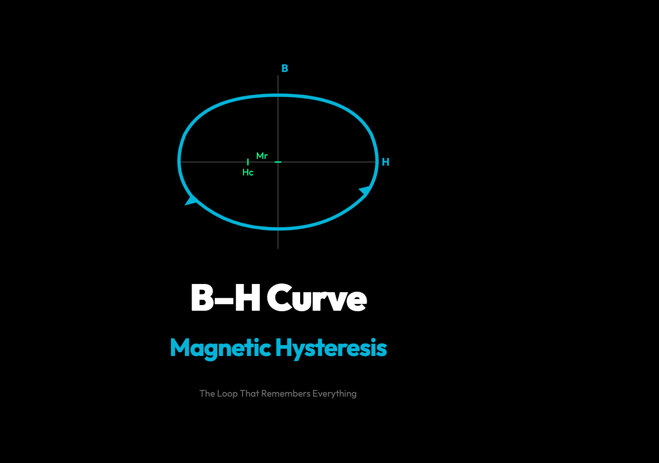
The standard way to visualize hysteresis is the B–H curve — a plot of magnetic flux density B against the applied magnetic field H. Start with demagnetized iron and steadily increase H, and B rises along a curved path toward saturation, where every magnetic domain in the material is aligned. This is the initial magnetization curve.
Now reverse the field. B does not retrace that curve. Instead it lags behind, and even when H reaches zero, B still holds a positive value — the remanent magnetization Mr, sometimes called the remanence or residual magnetization. This is the magnetic memory in action: the material is still partially magnetized even with no external field applied.
Keep reversing H, and eventually B reaches zero. The field at which this happens is the coercive force Hc — the amount of reverse field needed to wipe the material’s memory clean. Continue to strong negative saturation, then reverse again, and you trace a closed loop. That loop is the hysteresis cycle, and its area is not just a shape — it is a direct measure of energy lost as heat per complete magnetization cycle.
Why It Exists: Magnetic Domains
The microscopic origin of hysteresis lies in magnetic domains — small regions within a ferromagnetic material where atomic magnetic moments all point in the same direction. In an unmagnetized piece of iron, these domains are arranged randomly, canceling each other out macroscopically.

When you apply an external field, domains aligned with the field grow at the expense of others. This domain wall motion is not frictionless — it occurs through nucleation, pinning, and release that depends on the material’s crystalline defects and grain boundaries. Those imperfections act as pinning sites that hold domain walls in place even after the external field is removed. That pinning is what creates the lag, and it is why hysteresis is inherent to real materials rather than an artifact of measurement.
The Jiles-Atherton model, widely used to describe soft magnetic materials, captures this with five parameters: saturation magnetization Ms, domain wall density a, interdomain coupling alpha, pinning strength k, and magnetization reversibility c. Each one shapes the loop’s width, height, and curvature — and engineers select materials by their hysteresis parameters, not just their saturation values.
The Energy Cost of a Cycle
Perhaps the most consequential consequence of hysteresis is the energy dissipated per cycle. The area enclosed by the B–H loop has units of joules per cubic meter — energy density. In a transformer core cycling at 50 or 60 Hz, that energy loss appears as heat hundreds of times per second. The core losses from hysteresis alone are proportional to the frequency and the area of the loop.
This is why electrical steel used in transformer cores is not pure iron — it is carefully alloyed grain-oriented steel designed to minimize the hysteresis loop area. The same physics that creates magnetic memory also determines how much power a transformer wastes. Engineers call materials with narrow loops “soft” magnetic materials (low coercivity) and those with wide loops “hard” magnetic materials (high coercivity). The difference is the hysteresis loop.
Two Ends of the Same Curve
The practical applications of hysteresis are defined by which part of the curve you exploit:
Soft magnetic materials (transformer cores, electric motor laminations) have narrow hysteresis loops — low coercivity means they magnetize and demagnetize easily with minimal energy loss. The tradeoff is that they do not retain magnetization once the external field is removed.
Hard magnetic materials (permanent magnets, refrigerator magnets, magnetic recording media) have wide hysteresis loops — high coercivity means they hold their magnetization against demagnetizing fields. The tradeoff is that they are difficult to magnetize in the first place.
Every electric motor, generator, transformer, and hard drive in the world depends on this distinction. A hard disk stores data by magnetizing tiny regions in one of two directions — the wide hysteresis loop ensures those magnetizations do not decay when power is off. An electric motor uses soft magnetic material in its core to route magnetic flux with minimum energy loss.
The hysteresis loop isn’t just a curve on a graph — it’s a memory trace written into every piece of iron, cobalt, and nickel in the world. Each time you cycle a magnetic material through a magnetic field, the loop area tells you exactly how much energy the material absorbed and released as heat. That energy loss is why transformers hum, why permanent magnets have a lifespan, and why geologists can read the history of ancient rocks from their magnetic domains.
The real surprise is that this memory property, which seems like a limitation, is exactly what makes permanent magnets useful. Without hysteresis, there would be no refrigerator magnet, no hard drive, no compass needle. The same physics that makes some materials “forget” also makes others remember — and that distinction shapes nearly every piece of electrical infrastructure in the modern world.
What the Interactive Simulation Shows
The magnetic hysteresis simulation lets you apply a varying external field and watch the B–H curve trace its characteristic loop in real time. You can adjust the saturation magnetization, coercive force, and remanence to see how each Jiles-Atherton parameter changes the loop’s shape. Increasing the pinning parameter k widens the loop and increases energy loss per cycle. Reducing it narrows the loop toward the ideal soft-magnet behavior.
Notice that when you reduce the field to zero from saturation, the B value does not drop to zero — it stops at the remanence point on the vertical axis. That vertical gap is the material’s memory of having been saturated. The only way to return B to zero is to apply a reverse field of at least the coercive force Hc.
This is the fundamental asymmetry of hysteresis: the path from saturation to zero coercivity is not the same as the path from remanence to any given field value. The material’s state depends on which direction you approached it from.
Why This Matters
The hysteresis loop is one of the most practically consequential curves in all of physics. It determines how much energy a transformer wastes, how long a permanent magnet lasts, how much data a hard drive can store, and why certain materials can hold information without power. The loop’s area is a direct readout of energy lost; its width is a measure of magnetic memory.
Without magnetic hysteresis, none of the electrical infrastructure that defines the modern world would function. Permanent magnets would not be permanent. Hard drives could not store data reliably. Motors would be far less efficient. The fact that a piece of iron can remember its past is not a bug — it is the feature that made our present possible.