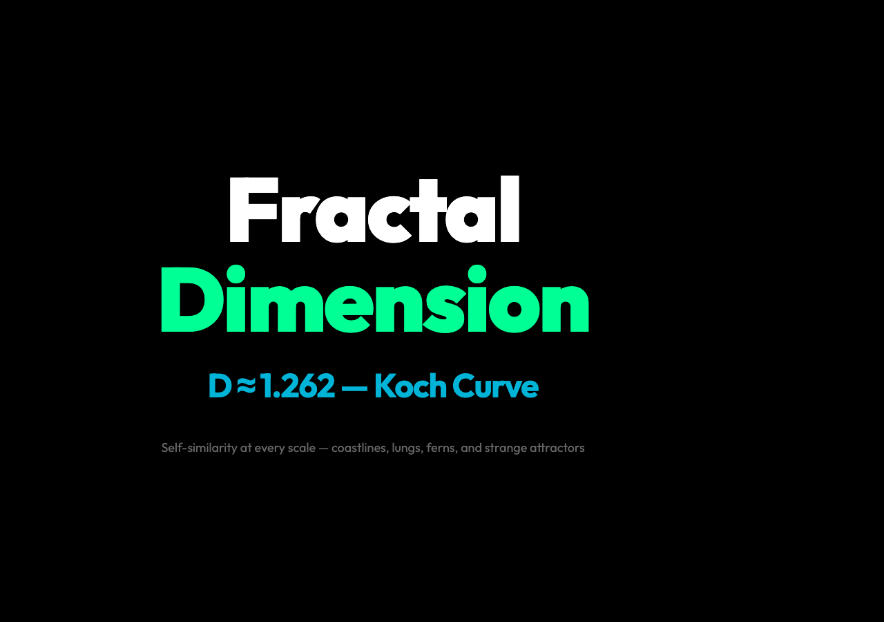
The Koch curve doesn’t just live in mathematics textbooks — it appears in the jagged edges of Norway’s coastline, in the branching pattern of your lungs, and in the structure of ferns that have been around for 360 million years. The dimension of a fractal isn’t an abstract curiosity; it’s a measurement that tells you how completely a shape fills the space it lives in. A smooth line fills space one way. The Koch curve fills space in a way that isn’t one-dimensional or two-dimensional — it occupies something in between, and that fractional dimension is how mathematicians characterize the difference. The implication is unsettling: the geometry of nature isn’t the smooth Euclidean geometry we were taught in school. It’s fractal, all the way down.
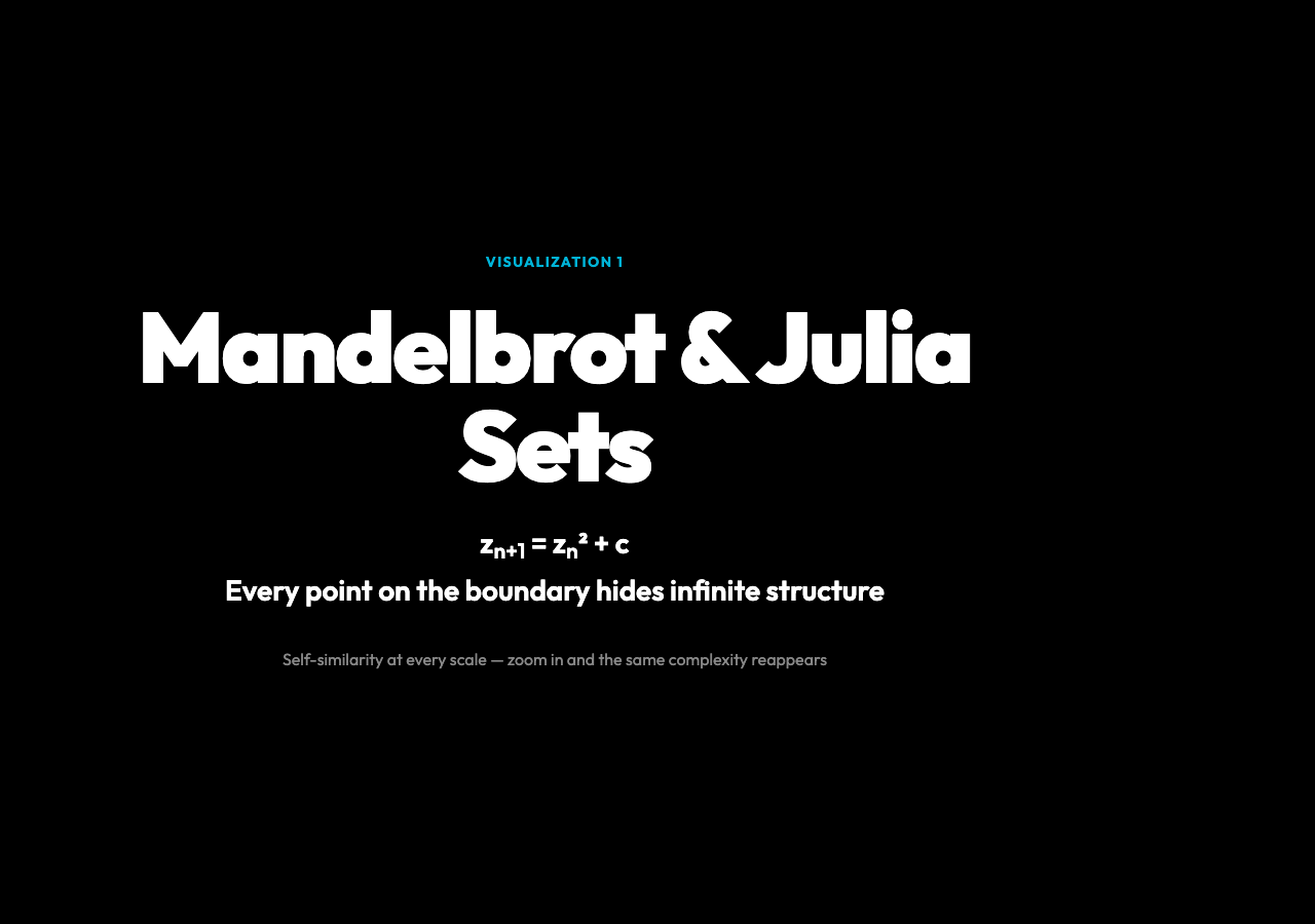
When Benoit Mandelbrot first viewed the set named after him on a computer screen in 1980, the pattern that emerged looked like a potato with infinite cauliflower growing from its edges. Zoom in anywhere near the boundary and the same complicated shape reappears — not exactly the same, but statistically self-similar. This property of self-similarity at every scale is what makes fractals both beautiful and deeply strange. It means no matter how much you zoom in, you’re never looking at something simpler. The complexity is built into the structure itself, not added from outside.
The mathematics behind the Mandelbrot Set is deceptively simple: take a complex number c, start with z_0 = 0, and repeatedly calculate z_{n+1} = z_n² + c. If the result stays bounded as you iterate, c belongs in the set. The entire shape emerges from this one formula applied across every point in the complex plane. There is no symmetry in the formula — only iteration — and yet the boundary produces infinitely intricate structure. That tension between simple rules and complex outcomes is the defining feature of chaotic dynamical systems, and it’s why fractals sit at the intersection of geometry, dynamical systems theory, and physics.
What makes the Mandelbrot Set especially striking is the Julia set. For each choice of the constant c, you get a different Julia set J_c — some connected, some Cantor dust (scattered fragments). The Mandelbrot set acts as a map of the parameter space: if c is inside the Mandelbrot set, J_c is connected; if c is outside, J_c is a Cantor set. This means the Mandelbrot set is not just a beautiful object — it’s a classification tool that tells you the global topology of an entire family of dynamical systems. This connection between a parameter map and the behavior of individual systems is the kind of structure that physicists and mathematicians find genuinely useful, not just aesthetically pleasing.
If the Mandelbrot and Julia sets show fractal structure in pure mathematics, the Barnsley Fern shows it in what looks like biological evolution. The fern is generated by an iterated function system — four affine transformations applied probabilistically. Each transformation has a weight: the stem accounts for 1% of the iterations, the leaflets for 85%, 7%, and 7% respectively. That 85% probability for the leaflets is not a design choice — it is the number that makes the fern look like a natural fern. Michael Barnsley discovered this by studying actual ferns and reverse-engineering the transformations that produce them. The result is a fractal that is statistically indistinguishable from its biological counterpart. The affine transformations encode the self-similarity through scaling, shearing, rotation, and translation — and the probabilities encode which branch gets which share of theiteration budget.
This IFS approach is structurally identical to how dynamical systems theory describes physical attractors. A strange attractor is a set in phase space toward which a dynamical system evolves. The Lorenz attractor — famous for its butterfly shape — has a fractal dimension of approximately 2.06, which tells you it occupies a volume in phase space that is not quite a surface but not quite a solid either. The dimension is a measurement of how the attractor fills its space, and for chaotic systems, this fractional dimension is often a key diagnostic. It tells you something concrete about the geometry of the chaos you are looking at.
The Fractal Tree visualization makes this concrete. Each branch splits into two at a fixed angle, and each child branch is a scaled copy of its parent. The number of branches follows N = 2^{depth+1} − 2, which grows exponentially with depth. At depth 7, you already have over 1,000 branches — each one a scaled copy of the whole. The formula N = 2^{depth+1} − 2 is not an approximation or a coincidence; it is a direct consequence of binary splitting. What looks like a living, growing tree in the visualization is just that formula made visible. Each branch is a self-similar copy of the entire tree at a smaller scale. This is fractal geometry made algorithmic.
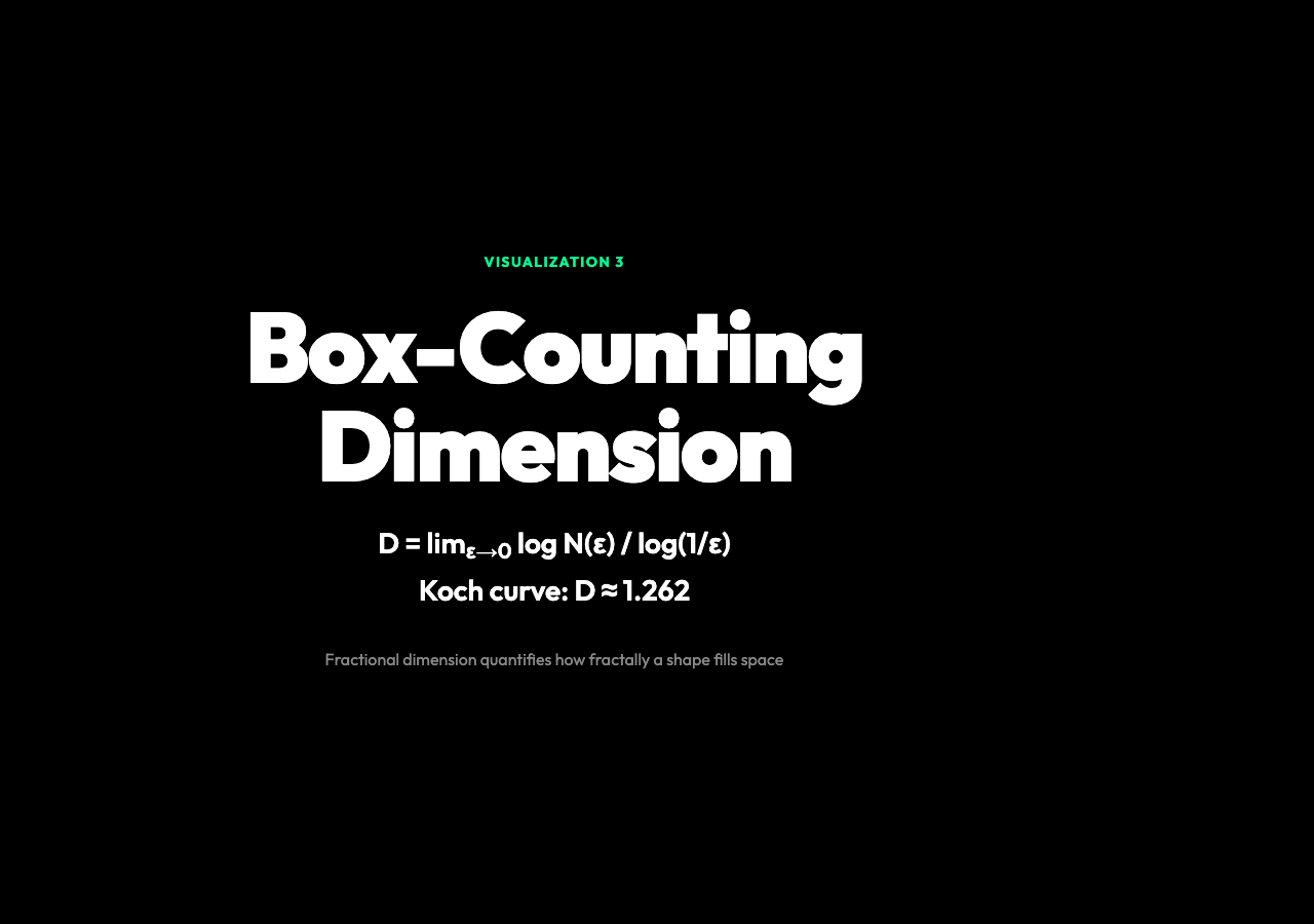
The Box-Counting Dimension ties the visual back to the quantitative. The idea is straightforward: cover the fractal with boxes of size ε, count how many boxes N(ε) contain part of the fractal, then compute D = lim_{ε→0} (log N(ε) / log(1/ε)). For a line, D = 1. For a filled square, D = 2. For the Koch curve, D ≈ 1.262. The Koch curve is longer than a line — it winds more in the same 1-dimensional space — but it doesn’t fill a 2-dimensional area, so its dimension sits between 1 and 2. The value of D is not arbitrary; it is a geometric invariant that tells you how efficiently the fractal fills space. Measuring D for a real coastline gives you a number that quantifies its jaggedness in a way that a simple length measurement cannot, because the measured length depends on the ruler size — a smaller ruler catches more detail and produces a longer measurement. The fractal dimension is the correction that makes the measurement stable.
This is why fractal geometry matters beyond its aesthetic appeal. Coastlines have fractal dimension around 1.2 to 1.3. Mountain ranges have fractal structure. Blood vessels in the human body branch fractally to maximize surface area within a constrained volume. Ferns use fractal branching to maximize light capture per unit of biomass. In every case, the fractal structure is not incidental — it is the solution evolution or geophysics arrived at for filling space efficiently under physical constraints. The mathematics and the natural phenomenon are not metaphorical parallels; they are the same geometry operating at different scales.
The Self-Similarity Test
The defining diagnostic of a fractal is statistical self-similarity across scales. In the Mandelbrot Set, zoom toward any point on the boundary and you find smaller copies of the larger structure — not identical, but following the same statistical pattern. In a fractal tree, each branch is a smaller copy of the whole tree. In a fern, each leaflet resembles the entire fern. Self-similarity is the fingerprint that identifies fractal structure. If you zoom in and the patterns change character entirely — becoming simpler rather than maintaining complexity — the shape is not fractal. The complexity must persist under magnification.
For the Barnsley Fern, self-similarity is encoded in the affine transformations. Each of the four transformations maps the whole fern to one of its parts: stem, upper leaflet, lower-left leaflet, lower-right leaflet. The IFS (Iterated Function System) is a set of contraction mappings, and the fixed point of the IFS is the fern itself. The mathematical structure — a fixed point of an iterated function system — maps directly onto what the fern looks like and how it grows. The fractal is a fixed point of a dynamical process. This is not metaphor; it is the same vocabulary used in dynamical systems theory for physical attractors.
Chaos and Dimension
Chaotic systems and fractals are deeply intertwined. The Lorenz attractor, one of the earliest and most famous chaotic dynamical systems, has a fractal dimension of approximately 2.06. The attractor is a surface in phase space — but a surface that is nowhere smooth, folding infinitely on itself. Its dimension slightly above 2 reflects this: it is almost a 2D surface but has enough “thickness” to fill slightly more than two dimensions. The fractal dimension of a strange attractor characterizes the geometry of chaos itself — how the trajectories pack in phase space and how sensitive the system is to initial conditions.

The connection goes both directions. Many chaotic systems have fractal attractors. Many fractals — including the Mandelbrot and Julia sets — arise from iterating simple nonlinear maps. The chaos is in the dynamics; the fractal is in the geometry of the limit set. The box-counting dimension gives you a way to put a number on that geometry. For the Julia set at a typical parameter value, the dimension is either 2 (connected Julia set) or somewhere between 1 and 2 (Cantor Julia set). The transition between these two regimes happens at the boundary of the Mandelbrot set. Where the parameter c sits — inside or outside — determines the topology of the resulting fractal. This is why the Mandelbrot set is both beautiful and structurally important: it is a bifurcation diagram for the family of quadratic polynomials z² + c.
What Fractal Dimension Actually Measures
The box-counting dimension is a limit, and like all limits in analysis, it is definitionally resistant to direct computation. In practice, you estimate it by covering the fractal with boxes at several scales ε, plotting log N(ε) against log(1/ε), and measuring the slope. The slope is the estimated fractal dimension D. For a perfect self-similar fractal like the Koch curve, the theoretical value D = log 4 / log 3 ≈ 1.262 is known analytically. For coastlines and natural structures, you estimate D from data. The slope tells you how the measure — the number of boxes — scales with resolution. A higher D means the shape fills space more efficiently at small scales. Coastlines with D ≈ 1.3 are more jagged than those with D ≈ 1.1.
This is the key insight: the fractal dimension is resolution-independent in a specific sense. A small ruler produces a longer measured length for a fractal than a large ruler, so raw length is resolution-dependent. The fractal dimension corrects for that dependence by quantifying how the measured length (or area, or volume) scales with the measurement resolution. Two coastlines with the same measured length at one scale may have different fractal dimensions, reflecting different underlying jaggedness. The dimension is a stable property; the raw measurement is not. When you see a result like “fractal dimension of human brain gray matter is approximately 2.73,” that number is not an accident — it reflects the scaling structure of cortical folding, and it is measurably different from the fractal dimension of other organs.
The Takeaway
Fractal geometry is not a mathematical curiosity living in research papers — it is the actual geometry of natural systems. The Koch curve with its D ≈ 1.262, the Barnsley Fern with its four IFS affine maps, the Mandelbrot set with its z² + c iteration and the Julia sets it parameterizes: these are the models that describe how coastlines fracture, how lungs branch, how ferns grow, and how strange attractors fold in phase space. The fractional dimension is the quantification that makes fractal structure legible to measurement. And because self-similarity appears at every scale in natural systems — not as an approximation but as a structural feature — fractal geometry is not an exotic alternative to Euclidean geometry; in many cases, it is the more accurate description.
Try the Fractal Chaos Systems visualization to explore the Mandelbrot set, Julia sets, Barnsley Fern, and box-counting dimension interactively — or see live examples of fractal behavior across different parameter settings.