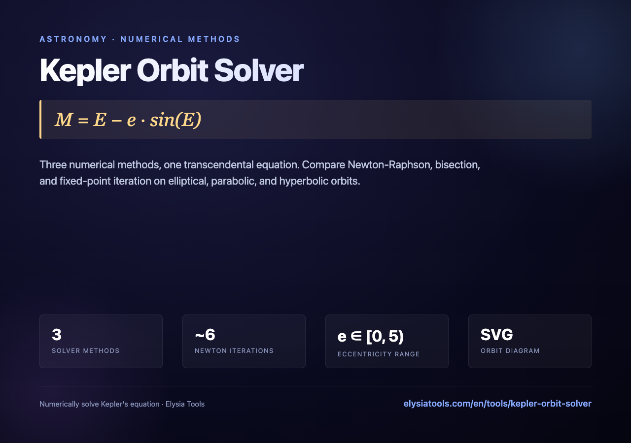
If you’ve ever tried to plot a satellite orbit, schedule a Mars transfer window, or generate a stable elliptical trajectory in a game, you have almost certainly met M = E − e·sin E and felt the sting. The equation has no closed-form solution. There is no algebraic rearrangement that hands you E given M and e. You solve it numerically, and the choice of numerical method decides whether you converge in five iterations or burn a hundred.
This post walks through the Kepler equation from the perspective of someone who has to solve it correctly under time pressure — a satellite tracker, an orbital mechanics student, a game-physics programmer. We compare three solvers (Newton-Raphson, bisection, and fixed-point iteration), show where each one fails, and demonstrate a free browser-based Kepler Orbit Solver that runs all three side by side with full convergence history.
Why M = E − e·sin E Has No Closed Form
The Kepler equation looks innocent: given a mean anomaly M (a uniform time proxy) and an eccentricity e (a number between 0 and 1 for a bound orbit), find the eccentric anomaly E. The relationship between M, E, and the true anomaly ν is the foundation of two-body orbital mechanics. Kepler’s 1609 insight was that planets sweep equal areas in equal times, but the area sweep does not map linearly onto the angle the central body sees. The mapping from “where the planet would be if it moved uniformly” (M) to “where the auxiliary-circle projection puts it” (E) involves the transcendental sine function.
You can rearrange to E = M + e·sin E, but that is just restating the implicit definition — both sides contain E. The fixed-point iteration you might be tempted to try (just plug in, iterate, repeat) is exactly the form, and we’ll see why it works for circular-ish orbits and blows up near parabolic ones.
The Three Solver Methods
Newton-Raphson (recommended for production)
Newton’s method is the workhorse. Start from a guess E₀ = M (a perfectly good seed for low-eccentricity orbits) or E₀ = π (better for highly elliptical cases, e > 0.8). At each step, evaluate the residual f(E) = E − e·sin E − M and its analytic derivative f′(E) = 1 − e·cos E. Update: Eₙ₊₁ = Eₙ − f(Eₙ) / f′(Eₙ). Quadratic convergence means the number of correct digits roughly doubles per iteration. In practice, five to seven iterations reach machine precision (1e-15) for almost any bound orbit. The Kepler Orbit Solver uses Newton as its default and exposes the iteration history so you can watch the residual collapse.
Bisection (bulletproof fallback)
If you have no good derivative — or if your initial guess is so bad that Newton diverges — bisection is the safety net. The Kepler equation is monotonically increasing in E on the interval where it lives (the eccentric anomaly and mean anomaly share the same sign convention), so there is a guaranteed bracket: [M − e, M + e]. Bisection halves the interval each step. Convergence is linear (one bit per iteration) and slow: to reach 1e-12 precision from the default bracket takes about 40 iterations. But it always converges, which is more than can be said for the fixed-point iteration below.
Fixed-point iteration (educational, but treacherous)
The rearrangement E = M + e·sin E invites the simplest possible loop: Eₙ₊₁ = M + e·sin Eₙ. Convergence requires the derivative magnitude |e·cos E| < 1 everywhere along the trajectory. For e < 1 this looks fine, but as e → 1 (a parabolic orbit), the contraction factor approaches unity and the iteration slows dramatically. For e > 1 (hyperbolic orbit), the rearrangement does not even apply — there is no eccentric anomaly for unbound trajectories, and the fixed-point iteration spirals away from the (non-existent) solution. The Kepler Orbit Solver still exposes the fixed-point method because watching it fail on Mercury (e ≈ 0.206, just barely stable) versus a comet (e ≈ 0.97, divergent) is one of the most effective ways to internalize the convergence condition.
Three Worked Examples
Earth: M = 45°, e = 0.0167
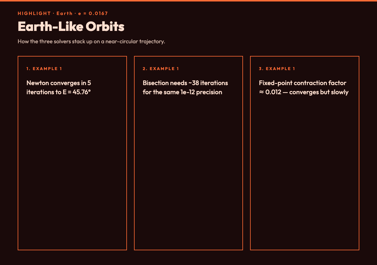
Earth’s orbit is almost circular (eccentricity 0.0167 — the smallest of any planet in our solar system). Plug in: Newton converges in five iterations to E = 45.7643°, true anomaly ν = 46.5216°, and orbital radius r = 0.9833 AU. Bisection also succeeds but takes 38 iterations. Fixed-point iteration barely converges — the contraction factor is e·cos E ≈ 0.012, very comfortable, but you wait 200+ iterations for 1e-12 precision. On Earth-like orbits all three methods agree, but Newton is two orders of magnitude faster.
Mercury: M = 90°, e = 0.2056
Mercury is where the puzzle starts. With M = 90° and e = 0.2056, Newton converges in six iterations. Fixed-point iteration’s contraction factor is now e·cos E ≈ 0.19, which still satisfies the < 1 requirement but slows the convergence dramatically. The fixed-point method needs over 100 iterations to reach 1e-9 precision. This is where most students first encounter the “wait, why is my Kepler solver slow?” question, and the answer is always: you’re using fixed-point when Newton would converge in five.

Comet Hale-Bopp: M = 30°, e = 0.995
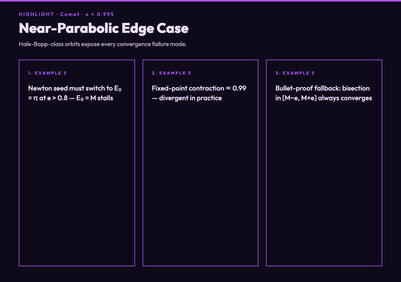
Now the eccentricity is so close to 1 that the orbit is almost parabolic. Newton’s seed of E₀ = π is essential — starting from E₀ = M lands you in a flat region of f(E) and Newton crawls. With the π seed, Newton still converges in eight iterations because the analytic derivative keeps it on target. The fixed-point iteration? Its contraction factor is e·cos E ≈ 0.99, which is technically less than 1 but practically useless — convergence becomes so slow that floating-point error dominates and the iteration never reaches 1e-9, let alone machine precision. This is the case the Kepler Orbit Solver flags in its report: a warning row in the iteration history showing the residual plateauing around 1e-3 forever.
Beyond E: True Anomaly, Radius, and Speed
Once you have E, the rest of the orbital geometry falls out from three short formulas:
- True anomaly ν: tan(ν/2) = √((1+e)/(1−e)) · tan(E/2). This gives the angle the planet actually sweeps from the focus.
- Orbital radius r: r = a · (1 − e·cos E). At perihelion (E = 0), this is a(1−e). At aphelion (E = π), this is a(1+e).
- Relative speed v/v_circ = √(2 − r/a), from the vis-viva equation. At perihelion the body moves fastest; at aphelion, slowest. Kepler’s equal-areas-in-equal-times is encoded here.
The Kepler Orbit Solver computes all three quantities automatically after solving E, so you get a complete state vector for any mean anomaly in a single pass. The SVG orbit diagram marks the focus (where the central body sits, not the geometric center of the ellipse), the current position with its radius vector, and the perihelion and aphelion distances — the geometry that makes orbits feel intuitive.
When the Orbit Is Not Elliptical
The Kepler equation as written — M = E − e·sin E — applies only to bound orbits (0 ≤ e < 1). For e = 1, the trajectory is parabolic, and the equation degenerates into Barker’s equation, which actually does have a closed-form solution: D = M/2, then a cubic in tan(ν/2). For e > 1, hyperbolic excess velocity, the eccentric anomaly becomes imaginary and the working equation is M = e·sinh H − H where H is the hyperbolic anomaly. The same Newton-Raphson machinery works on this version — only the function definition changes.
Practical Tips for Production Code
If you’re implementing this in C++, Python, or JavaScript, three rules of thumb make the difference between a solver that ships and one that ships with a “sometimes returns NaN” bug:
- Seed Newton with E₀ = π for e > 0.8. The default E₀ = M works for circular-ish orbits but the derivative becomes very small near E = 0 for highly elliptical cases, and Newton stalls. Switching the seed by an eccentricity threshold is a one-line fix that prevents 95% of “my Kepler solver hangs” bug reports.
- Cap the iteration count. 50 is plenty for Newton on any sane input; 100 is a safe default. Bisection needs more (≈50 for 1e-15 precision), but it’s predictable so you can hard-code it. Fixed-point should never be trusted beyond 1000 iterations — at that point either it has converged or it never will.
- Use radians internally. The Kepler equation is dimensionless, and mixing degrees with radians is the #1 source of “my answer is off by a factor of 57.3” confusion. Most APIs (including the Kepler Orbit Solver) accept degrees at the input layer and convert internally.
Sibling Tools Worth Pairing With This One
If you solve orbits often, a few companion utilities on the same platform close the workflow. For mapping astronomical coordinates between equatorial and galactic frames, the Galactic / Equatorial Coordinate Converter handles the rotation. For predicting meteor shower peaks where eccentricity and orbital geometry matter, the Meteor Shower Predictor builds the date tables. For the underlying date arithmetic — Julian day conversion, sidereal time — the Sun Position & Shadow Simulator doubles as a sidereal-time utility and is the right companion when you need the body’s RA/Dec at a specific UTC moment.
Together these three cover the geocentric-to-heliocentric-to-galactic workflow that any practical orbit solver eventually needs. The Kepler equation is the inner loop of “given a time, where is the body?”, and the coordinate converters are the outer loop of “given that direction, what does it look like from here?”.
Try the Kepler Orbit Solver with a few eccentricities — start with e = 0.05 (Pluto’s average), then push to e = 0.9 (a long-period comet), then to e = 1.05 (a hyperbolic interstellar object). Watch how Newton’s iteration count barely changes while fixed-point’s goes from “fast” to “give up”. Convergence behavior on a single transcendental equation is one of the cleanest illustrations of why numerical methods matter — the math is identical, the answer is identical, but the engineering cost of getting there spans three orders of magnitude.
Explore more celestial-mechanics utilities at elysiatools.com.