The Half-Life Equation, Five Ways: A Field Guide to Exponential Decay

A package of iodine-131 arrives at the clinic. The dose calibrator reads 100 MBq. By the time the patient is ready, it reads 92 MBq. By lunch, 84. By tomorrow, 71. The same clock is running whether the clock is a hot cell in nuclear medicine, a dose-response curve in pharmacology, or the carbon-dating lab in an archaeology department. Three different vocabularies — isotope, drug, artifact — share one underlying equation: N(t) = N₀ · e^-λt.

The math is small. The trap is not doing it. Most half-life mistakes come from confusing the decay constant with the half-life, mixing the steady-state equation for repeated dosing with the single-dose equation, or dividing by 2 when you should be multiplying by e. A good calculator enforces the right form for each question. The Half-Life Calculator at elysia-tools.com is one of those tools: it doesn’t just compute, it picks the right equation for what you’re actually asking.

One equation, three different questions

Radioactive decay, drug elimination, and carbon-14 dating all reduce to the same differential equation. The differences are in the inputs and in what you’re trying to extract.

• Given half-life, find remaining amount. N(t) = N₀ · (½)t / T½. Carbon-14 with T½ = 5,730 years and a 10,000-year-old bone: N(10000) = N₀ · 0.298. About 30% of the original C-14 is left.
• Given remaining amount, find half-life. Solve the same equation for T½: T½ = t · ln(2) / ln(N₀ / N(t)). A 5 mg dose falls to 2 mg in 6 hours — that’s a 4.39-hour half-life drug.
• Given a target fraction, find time. t = T½ · ln(N₀ / N_target) / ln(2).

The unifying constant is the decay rate λ = ln(2) / T½. Once you know λ, every other quantity follows. The Exponential Calculator at the same site is the right tool when λ and t are already in hand and you just need e^-λt; the half-life tool is the right tool when T½, t, and amount are the inputs.

The radioactive-decay view: isotopes, units, and the daughter problem

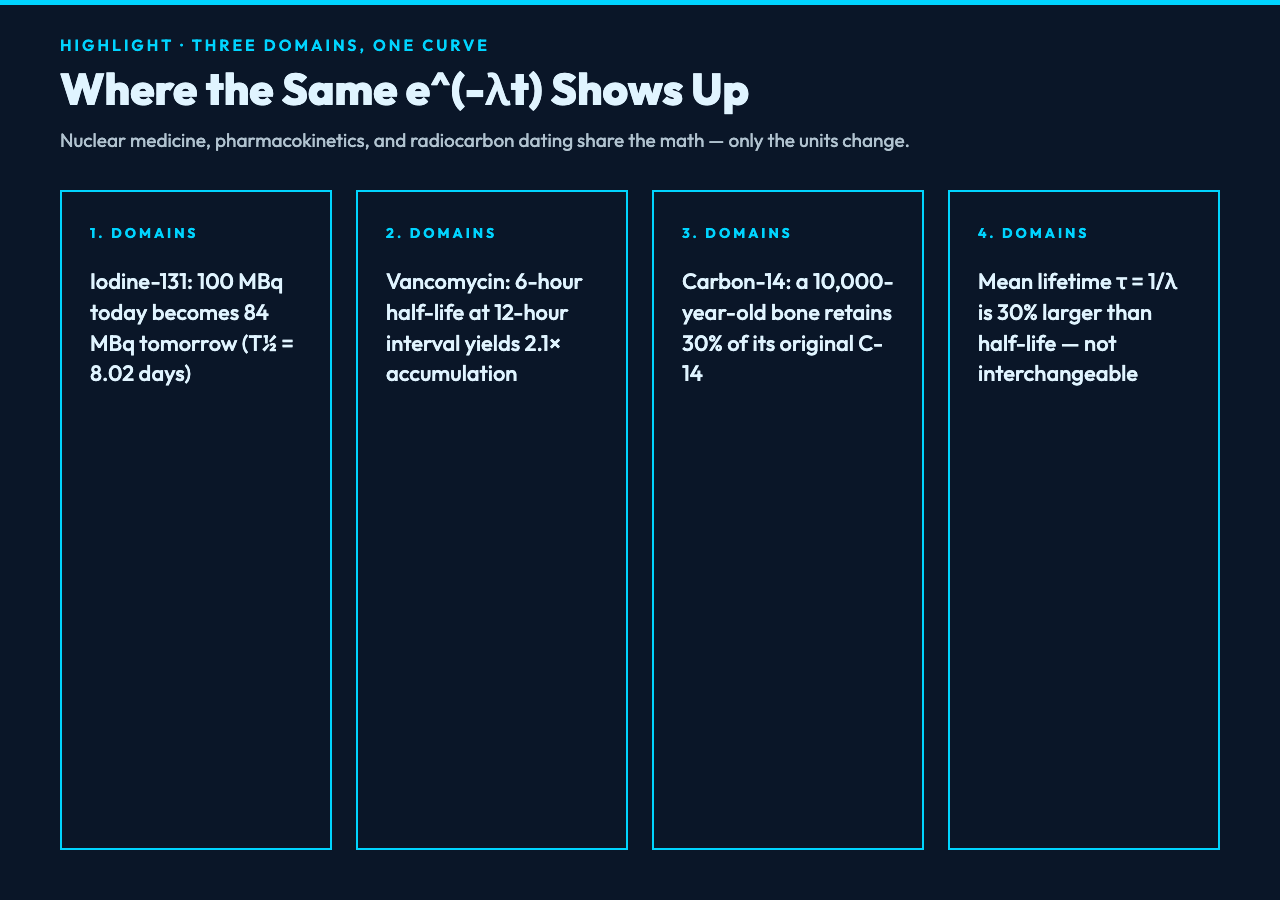
For a clinical isotope, the dominant question is what activity will this sample have when I use it? Iodine-131 has T½ = 8.02 days. A 100 MBq calibration on Monday yields 91.7 MBq on Tuesday, 84.0 on Wednesday, 77.0 on Thursday. The decay factor each day is e^-λ = 0.917. After ten days, the same sample is 41.6 MBq.

The tool makes the units explicit: input in hours, days, or years; output in becquerels, curies, or a fraction of the original. That sounds obvious until you watch a technologist divide MBq by 2.5 to “calibrate for ten days” — that’s three half-lives, not one, and the real remaining activity is 12.5%, not 40%.

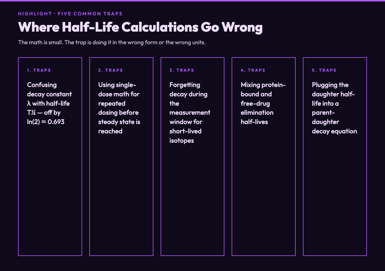
The daughter-product problem is where a calculator earns its keep. I-131 decays to Xe-131 (stable). I-125 decays to Te-125 (also stable). Cs-137 decays to Ba-137m, which then decays to Ba-137 with its own 2.55-minute half-life. For a parent-daughter pair, the apparent activity of the daughter depends on the parent’s half-life, the branching ratio, and the time since the parent was last separated. Plugging only the daughter half-life into the half-life tool is the classic mistake. The right move is to use it for the parent curve and to recognize that the daughter reaches a transient equilibrium that decays at the parent’s rate.

The pharmacokinetics view: why dosing schedules look the way they do

A drug with a 6-hour half-life given every 24 hours reaches steady state when the dose interval covers four half-lives. The accumulation ratio is 1 / (1 − e^-λ·τ), where τ is the dosing interval. For τ = 24 h and T½ = 6 h, that’s 1 / (1 − e^-4·ln(2)) = 1 / (1 − 0.0625) ≈ 1.067. The peak-to-trough ratio for that same drug at steady state is e^λ·τ ≈ 16, which is why every 6-hour drug has a flat plasma curve and every 24-hour drug has a 16× swing.

The half-life tool handles the steady-state accumulation problem directly: given a dose, dosing interval, and half-life, it returns the steady-state C_max, C_min, and average concentration. The same tool also solves the inverse: given a target trough level and a half-life, what dose and interval produce it?

Vancomycin is the standard teaching example. With T½ ≈ 6 hours in normal renal function and a 12-hour dosing interval, the accumulation ratio is about 2.1× and the trough is 50% of the peak. In renal failure the half-life stretches to 40-70 hours; the same 12-hour interval now produces an accumulation ratio above 4×, and the dosing interval has to widen to match. The numbers are not aesthetic — they drive the nomograms in clinical chemistry.

The archaeology view: when the date is older than your career

Radiocarbon dating is half-life math applied to the past rather than the future. The relevant half-life is the Libby half-life of 5,568 years (Cambridge half-life 5,730 ± 40 years — modern convention uses 5,568 for back-compatibility). A 1,000-year-old sample has lost 12% of its C-14. A 10,000-year-old sample has lost 70%. Beyond about 50,000 years (nine half-lives) the remaining C-14 is below 0.2% and measurement noise dominates.

The half-life tool isn’t a dedicated dating tool, but it’s the right sanity check on any carbon-date you read. Given a calibrated date range, ask the tool what fraction of C-14 should remain, then compare with the lab’s measurement. The lab does the curve fitting; the tool tells you whether the fitted curve is on the right track.

Five traps the calculator closes for you

1. Confusing λ with T½. The decay constant λ has units of 1/time; the half-life T½ has units of time. They differ by a factor of ln(2). A spreadsheet that takes one as input to the other’s equation is off by 0.693.
2. Mean lifetime vs half-life. The mean lifetime τ = 1/λ is larger than T½ by exactly ln(2) ≈ 30%. They’re not interchangeable.
3. Steady-state vs single-dose math. The accumulation ratio 1/(1 − e^-λτ) only applies after roughly 5 half-lives of consistent dosing. Before steady state, the equation for a single dose still applies, with the dose history summed.
4. Decay during the measurement. A 5-minute lung scan with Tc-99m (T½ = 6 hours) starts at the calibration activity but counts at the average. Short isotopes need a decay correction factor for the measurement window itself.
5. Saturation and protein binding. Pharmacokinetic half-life is the elimination half-life, not the receptor occupancy half-life. A drug that binds 99% to plasma protein behaves differently than the same free fraction in a buffer.

Putting it together

The half-life equation is a small piece of math, but it’s also one of the most cross-disciplinary pieces of math a working scientist touches. The same e^-λt shows up in nuclear medicine, in dosing schedules, in radiocarbon dating, in exponential distribution survival analysis (the Exponential Distribution Calculator uses it for memoryless waiting times), in capacitor discharge curves, and in any system where a constant fraction of the remaining quantity is lost per unit time.

The right tool does not just compute; it picks the right form. The Half-Life Calculator at elysia-tools.com handles the four common question shapes — given half-life find amount, given amounts find half-life, given target find time, given dosing schedule find steady-state levels — and lets you mix units (Bq/Ci, h/d/y) without dropping the conversion factor. It also exposes λ and τ explicitly, so the audit trail of any computation is visible.

For more tools in the same family, the Exponential Calculator covers the e^x/e^-x view, and the Exponential Distribution Calculator covers the probability side. Browse the rest of the Math & Numbers cluster for stoichiometry, thermodynamics, kinematics, and the other half-life-adjacent calculators that share the same exponential-decay backbone.