A high R-squared feels like a verdict. The number comes back at 0.92, the slope looks reasonable, and the chart goes into the quarterly review with the quiet confidence that the model “explains” the data. But R-squared is not a verdict. It is a contract — and you signed it without reading the diagnostics on the back page.
The number that everyone quotes and nobody interrogates
Most teams I have watched run a regression treat R-squared the way a wine list treats the vintage year — as a mark of quality to be recited, not interrogated. Coefficient of determination. Proportion of variance explained. The textbook definition is tight; the casual usage is loose, and the loose usage is where the trouble starts. R-squared tells you how well your chosen line fits your chosen data using your chosen features. It does not tell you whether the line is the right line, the data is the right data, or the features are the right features. Three distinct failure modes, all dressed up in the same number.
I once watched a marketing analyst defend a quarterly forecast to a CFO by holding up an R-squared of 0.94. The chart was beautiful. The chart was also built on six weeks of data, three of which were a Black Friday anomaly that no one flagged. When the next quarter rolled around and the forecast missed by twenty-two percent, the analyst did not say “the model was wrong.” She said, “we had a strange quarter.” The model had been strange the whole time. The number just hadn’t told her so.
This is the trap. R-squared is a single statistic summarizing a relationship the model fit to the points you handed it. Change any of the inputs — add a row, drop a row, swap a feature — and the number moves. The diagnostic question is not “what is my R-squared” but “what does my R-squared become when I break the inputs on purpose, and what does that tell me about the inputs I cannot break?”
Reading the diagnostics the line already gave you
The Regression Analyzer surfaces a stack of metrics that, taken together, build the case for or against your line. Five of them matter more than the rest, and each one is a sentence in the contract you signed with the data.
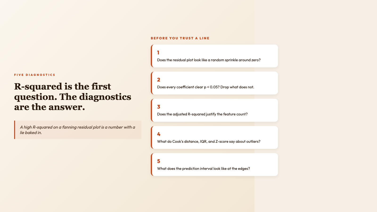
Residual plots. The single most underused diagnostic in business regression. Plot the residuals (the difference between each observed value and the value the line predicted) on the y-axis against the predicted values on the x-axis. If the cloud looks like a random sprinkle, your model has captured most of the signal. If the cloud fans out — narrow on the left, wide on the right — your model has a heteroscedasticity problem: the variance of the error depends on the value you’re predicting, and any confidence interval you report will be wrong at the tails. If the cloud curves — smile shape, U shape — your model is missing a nonlinear term and the linear fit is averaging over a wave. The R-squared on a fanning or curving residual plot is a number with a lie baked in.
Standard errors and p-values on the coefficients. Each coefficient in a multiple regression comes with a standard error that describes how much that coefficient would jitter if you redrew the sample. The t-statistic is the coefficient divided by its standard error; the p-value is the probability of seeing a t-statistic this large if the true coefficient were zero. A coefficient with a p-value above 0.05 is not “not significant” in some hand-wavy sense — it is statistically indistinguishable from no relationship at all. Reporting it as a driver anyway is a specific kind of mistake, and a particularly common one when analysts eyeball a slope and decide it “looks important.”
Adjusted R-squared. R-squared has a habit of going up whenever you add a feature, even a useless one. Adjusted R-squared penalizes the score for every feature you add, so a model that improves only by adding noise gets penalized back down. When comparing two candidate models with different numbers of features, adjusted R-squared is the fairer referee.
Outlier flags. A single high-leverage point — a row whose x-values are extreme — can pull a regression line across the chart like a magnet. Cook’s distance flags these points by measuring how much the line would shift if you deleted the row. The IQR rule (1.5 times the interquartile range) and the Z-score rule (more than three standard deviations from the mean) are two complementary ways to catch points that are unusual in y as well as in x. Whether to drop them, down-weight them, or report results with and without them is a domain decision. Hiding them is never the right call.
Confidence and prediction intervals. A confidence interval around a coefficient says “if I drew a thousand samples from this population, the true coefficient would land in this range ninety-five times out of a hundred.” A prediction interval around a new data point is wider — it has to cover both the uncertainty in the line and the scatter of individual points around it. The number on a forecast slide is almost always a point estimate. The interval around it is the honest version of the same forecast.
The five-question protocol before you trust a line
A regression that ships without these five questions answered is a guess with a chart on top.
- 1. What does the residual plot look like? A random sprinkle around zero means the model captured the structure. Anything else means the model is hiding a pattern it could not name.
- 2. Does every coefficient in the model beat a p-value of 0.05? If not, drop it and re-fit. Carrying an “almost significant” feature through a forecast is a tax you pay forever.
- 3. What is the adjusted R-squared, and does it justify the feature count? If a five-feature model has the same adjusted R-squared as a two-feature model, ship the two-feature model. Simpler is durable.
- 4. Are there high-leverage points, and what do the diagnostics say about them? Cook’s distance, IQR, Z-score — three flags, one decision: keep, drop, or report both.
- 5. What does the prediction interval look like at the edges of your data? A model trained on rows where x ranges from 10 to 50 should not be trusted at x = 200. Extrapolation is the silent killer of forecasts.
The Regression Analyzer walks through all five by default: residual diagnostics, p-values on each coefficient, adjusted R-squared alongside raw R-squared, IQR and Z-score outlier flags, and prediction intervals around the forecast. You can find it at elysiatools.com/en/tools/regression-analyzer, paste a CSV, set your target column, and the report appears in one tab. The earlier workflow — running the regression in one tool and the diagnostics in another — is what made R-squared the verdict instead of the question.
Where the tool earns its keep
Two scenarios show what the diagnostic-first workflow changes in practice.
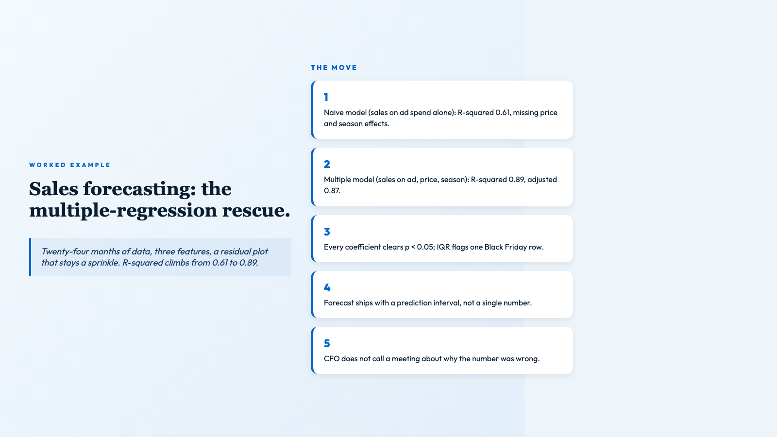
Sales trend forecasting. A marketing team uploads twenty-four months of monthly sales, with advertising spend, average price, and a season flag as features. The naive regression — sales on advertising alone — returns R-squared of 0.61. The multiple regression — sales on advertising, price, and season — returns R-squared of 0.89 and adjusted R-squared of 0.87. The residual plot is a random sprinkle; every coefficient clears p < 0.05; the IQR rule flags one Black Friday row; Cook’s distance agrees. The forecast for the next quarter includes a prediction interval. The team ships a range, not a point, and the CFO does not have to call a meeting about why the number was wrong. Worked examples for sales forecasting and quality-control optimization live on the CSV samples page — the input data is included so you can run the same analysis yourself in under a minute.
Quality control in a process plant. Process logs arrive with defect_rate as the target and temperature, pressure, and feed_rate as features. The first fit shows temperature with a p-value of 0.31. Drop it. Refit. The remaining two features clear p < 0.01, adjusted R-squared improves, the residual plot stays clean. The team now knows which two process parameters drive defects — not which three look like they might — and they can wire those two into the control loop.
A short list of things regression cannot do
The list is short on purpose, because every item is a category of mistake I have watched a team make.
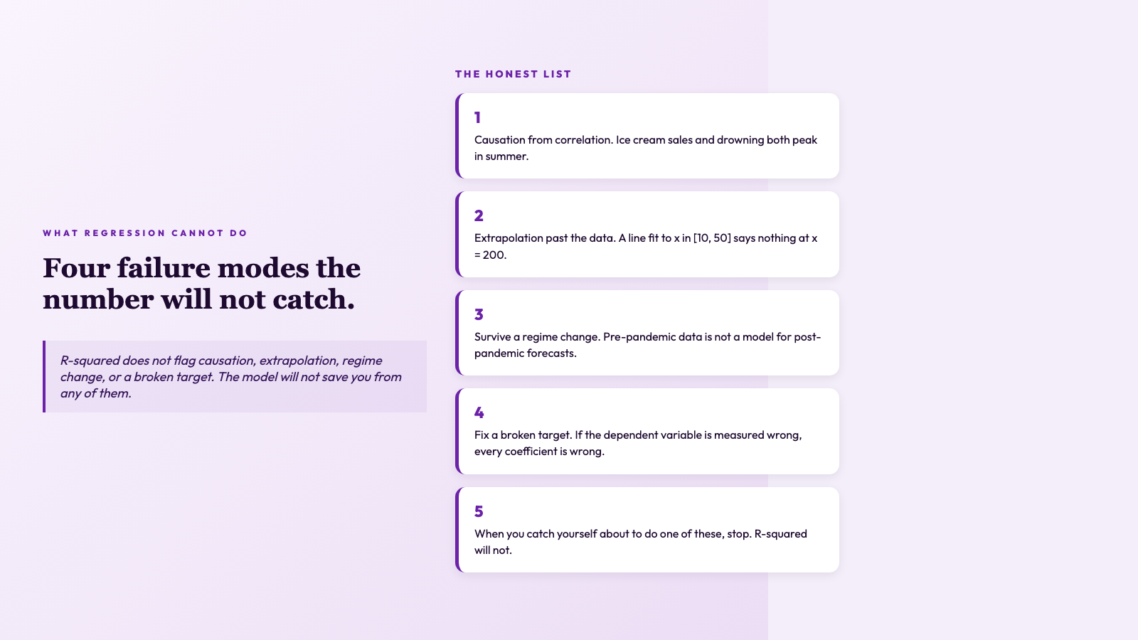
- – Establish causation from correlation. A regression line through ice-cream sales and drowning deaths does not mean ice cream kills people. Both are driven by summer.
- – Extrapolate past the training data. A line fit to x between 10 and 50 is not a line at x = 200. The model has no information there.
- – Survive a regime change. A model trained on pre-pandemic data is not a model for post-pandemic forecasts.
- – Fix a broken target. If the dependent variable is measured wrong, every coefficient downstream is wrong in proportion.
When you catch yourself about to do one of these, stop. R-squared will not catch you.
The closing move
A high R-squared feels like a verdict — but it is not. It is a contract between you and the assumptions you did not bother to write down. When the residual plot fans out, when one influencer point drags the line across the room, when your training data has twelve rows and three columns you forgot to standardize, the R-squared is still 0.92, and the prediction you ship is still wrong. The fix is not a cleverer algorithm. The fix is reading the diagnostics the model already gave you, then deciding whether the contract was honest. The Regression Analyzer prints every one of those diagnostics side by side — coefficients, standard errors, confidence intervals, residual plots, outlier flags — so the verdict and the doubts land in the same tab.
The tool is not the only thing you need. You also need the discipline to read the diagnostics it prints, the willingness to drop a feature that does not clear p < 0.05, and the honesty to report a prediction interval instead of a point estimate. The tool makes the discipline easy by putting every diagnostic on the same page, but it cannot make you read the page. Sample CSVs are available if you want to run a worked example end-to-end. If you would rather see the same analysis in a different shape, the Python samples walk through the same workflow with code, and the path analyzer samples show how the diagnostics pipeline reads when the inputs are messier than a textbook CSV.
R-squared is the first question, not the last. Ask it, then read the diagnostics, then ship the forecast with the prediction interval attached. The team that does this is the team whose models stop quietly lying. Explore more tools at elysiatools.com/en/tools.