
Trihybrid crosses are the point where most students stop drawing Punnett squares. The 8×8 grid has 64 cells, the phenotype ratio is 27:9:9:9:3:3:3:1, and the arithmetic errors creep in before you finish column three. The forked-line branch method is the clean alternative: each gene contributes a monohybrid ratio, and the final ratio is the product. Punnett Trihybrid & Dihybrid Cross Visualizer at Elysia Tools renders both views side by side, applies the right inheritance mode per gene, and returns the genotype and phenotype tallies that you can defend in a lab report. This field guide walks through the workflow, the three inheritance modes, the comparison between the grid and the branch method, and the failure modes that survive the click.
Why a 27:9:9:9:3:3:3:1 ratio is the wall, not the door
The textbook ratio is famous because it shows what happens when you multiply three independent monohybrid ratios that each follow 3:1 dominance. The classic derivation is correct, but the practical question is different. You have a real cross in front of you — YyRrCc crossed with YyRrCc — and you need to know which offspring phenotypes are recombinant, which are parental, and what proportion of each class to expect. A 64-cell square works on paper, but the moment one gene shifts to incomplete dominance you cannot just multiply the 3:1 ratios anymore, and the cell-by-cell method becomes the only defensible approach.
Punnett Trihybrid & Dihybrid Cross Visualizer at Elysia Tools is the tool that picks the right method for you. You declare each gene with its mode, you enter the parental genotypes, and the tool returns the full grid, the branch diagram, and the tallied ratios. The grid is generated cell by cell, so any combination of dominance modes is handled correctly, and the branch diagram is the same product-of-ratios shortcut that the textbook teaches — except the tool tells you the actual ratio when the modes are mixed, instead of pretending all three genes are complete dominance.
The forked-line method: when the shortcut is safe
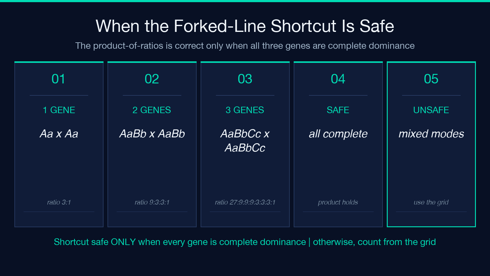
The forked-line (branch) method is the multiplication shortcut. For three independent genes each in complete dominance, the per-gene monohybrid ratio is 3:1, and the product is 27:9:9:9:3:3:3:1. You write each gene as a branch, multiply the probabilities along each path, and sum the paths that produce the same phenotype. The method is fast and produces the textbook ratio correctly when all three genes are complete dominance with non-overlapping alleles.
The shortcut breaks the moment one gene is incomplete dominance or codominance. A 1:2:1 monohybrid ratio that comes from an incomplete-dominance heterozygote (RW, pink, midway between red and white) does not produce a clean 3:1 phenotype ratio, and the multiplication product shifts. The cell-by-cell square still works — the dihybrid heterozygote cross gives 1:2:1:2:4:2:1:2:1 in pink-class merges, not 9:3:3:1 — and the tool falls back to the square whenever the modes are mixed. The branch diagram is rendered as a visualization, but the canonical tabulated ratio always comes from the grid.
Declaring genes: one line per trait, mode in brackets
The input format is one line per gene, with the trait name, an equals sign, the two alleles, and an optional mode in square brackets. The default mode is complete; the other choices are incomplete and codominance. A typical declaration for a textbook pea-seed dihybrid reads Seed color = Y,y and Seed shape = R,r, which is two lines and zero modes. The same cross with a snap-dragon-style flower color shifts to Flower = R,W [incomplete]. The tool matches the allele letters case-insensitively but keeps the casing you give — so AaBbCc and AABBCC and aabbcc all parse correctly, and the parent genotypes use the same letter conventions.
The tool supports two genes (dihybrid, 4×4 grid) and three genes (trihybrid, 8×8 grid). It does not support single-gene crosses — that is the dedicated Mendelian Punnett Square tool at Elysia Tools, which is the cleaner choice for one gene. The two-gene and three-gene cases are the entire point of this tool — single-gene problems do not need a visualizer, and the 4×4 to 8×8 jump is where most workflows start to drag.
The three inheritance modes and when each one bites
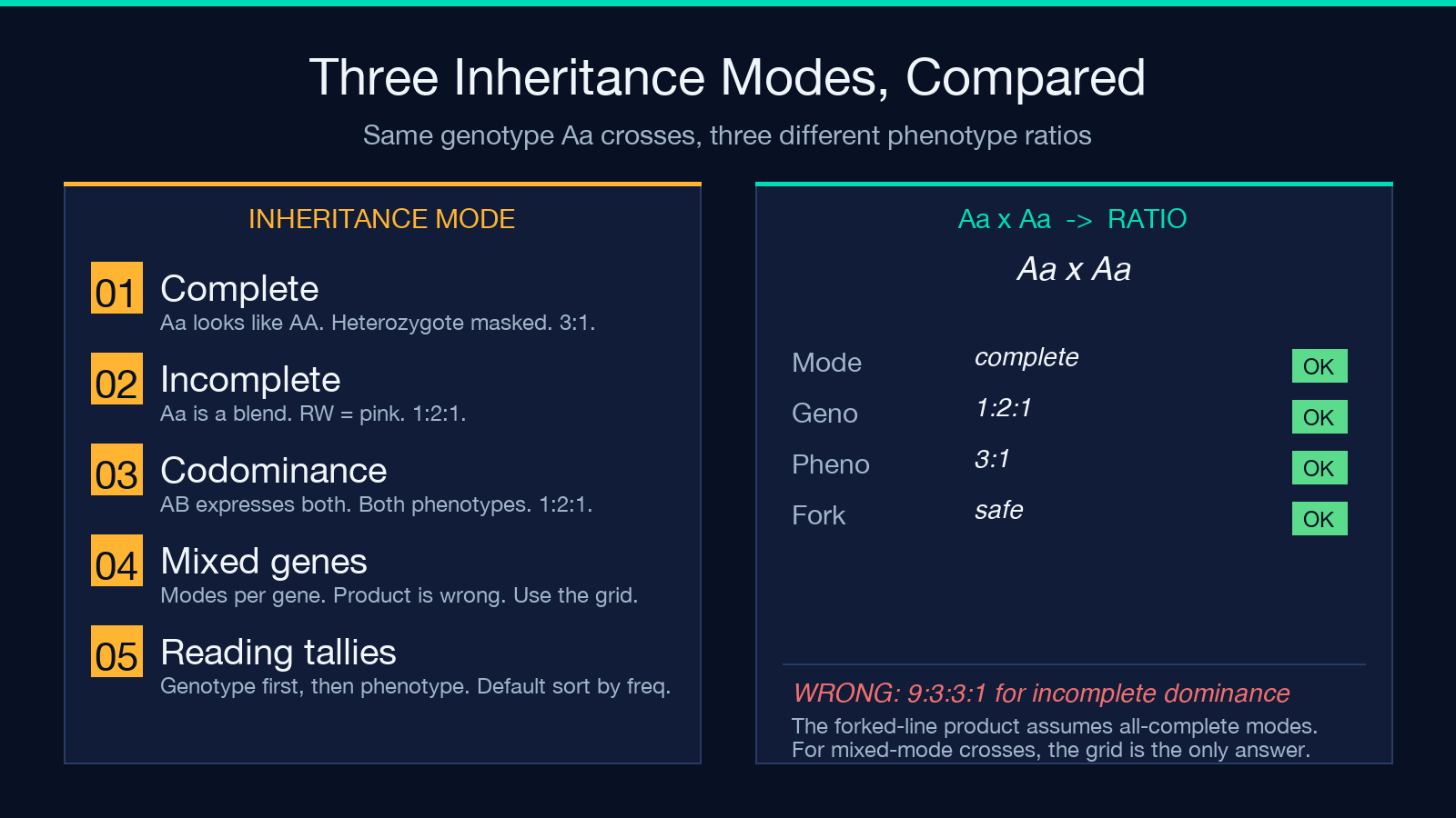
The mode attached to a gene line changes how the genotype translates to phenotype. The three modes are complete dominance, incomplete dominance, and codominance. Each one produces a different monohybrid ratio, and the combination of modes across the three genes is what determines whether the forked-line product is a valid shortcut.
Complete dominance. The uppercase allele masks the lowercase. Aa looks like AA phenotypically. The monohybrid ratio in a heterozygote cross is 3:1. The dihybrid phenotype ratio is 9:3:3:1. The trihybrid phenotype ratio is 27:9:9:9:3:3:3:1. Complete dominance is the textbook case and the only one where the forked-line product is correct without per-gene re-derivation.
Incomplete dominance. The heterozygote is a blend. RW produces pink, midway between red and white. The monohybrid ratio is 1:2:1 (red : pink : white), not 3:1. The dihybrid phenotype ratio is 1:2:1:2:4:2:1:2:1, not 9:3:3:1. The forked-line shortcut is unsafe here, and the tool’s grid is the source of truth.
Codominance. Both alleles express in the heterozygote. AB produces both A and B antigens (the classic ABO blood-type case). The monohybrid ratio is 1:2:1 like incomplete dominance, but the phenotype labels are distinct categories, not a blend. The forked-line product is correct when you treat each phenotype bin as its own category, but the tool still tallies from the grid to avoid the mode-mixing ambiguity.
What the output actually shows
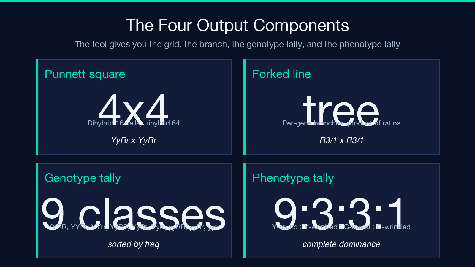
The output has four components. The Punnett square is the full 2^n by 2^n grid, with each cell containing the offspring genotype and the resolved phenotype. The forked-line diagram is the branch-method visualization, drawn as a tree with the per-gene monohybrid ratio at each branch and the product along each path. The genotype ratio is the tally of every unique genotype with count and percentage, sorted by frequency by default. The phenotype ratio is the same tally at the phenotype level, after applying each gene’s mode.
The display mode (both, square, or branch) controls which of the two visualizations is rendered. The both default is the right choice for teaching because students see the grid method and the branch method side by side, and the cross-check between them is the lesson. The square mode is faster to scan when the cross is large and the branch diagram would be more visual noise than help. The branch mode is the right choice for textbook derivation where the product-of-ratios is the argument.
Worked example: the classic YyRr dihybrid
The classic Mendel pea-seed dihybrid is the right starting case. Genes: Seed color = Y,y and Seed shape = R,r, both in complete dominance. Parents: YyRr and YyRr. The grid is 4×4 with sixteen cells, the genotype ratio covers nine distinct classes (YYRR, YYRr, YYrr, YyRR, YyRr, Yyrr, yyRR, yyRr, yyrr) and the phenotype ratio is 9:3:3:1 (yellow-round : yellow-wrinkled : green-round : green-wrinkled). The forked-line product gives the same 9:3:3:1. The two methods agree, the ratio is the textbook answer, and the tool is correct.
The same dihybrid with one gene in incomplete dominance is the case where the shortcut breaks. Genes: Seed color = Y,y and Flower = R,W [incomplete]. Parents: YyRW and YyRW. The grid is 4×4 with sixteen cells, the genotype ratio is the same nine classes, but the phenotype ratio is 3:6:3:1:2:1 (yellow-red : yellow-pink : yellow-white : green-red : green-pink : green-white). The forked-line product gives 9:3:3:1 if you ignore the mode, which is wrong. The tool’s grid is the source of truth, and the branch diagram is rendered with the per-gene mode-adjusted ratios so the visual matches the tabulated answer.
Limitations and what to do about them
The tool assumes unlinked genes. If two genes are linked (on the same chromosome with measurable recombination frequency), the independent-assumption multiplication is wrong, and the grid reflects independent assortment only. For linked genes, the dihybrid ratio shifts toward the parental classes — more AB/ab, less Ab/aB — and the tool does not currently take recombination frequency as an input. The workaround is to compute the linked ratio by hand and use the tool for the independent-correction visualization, or to bypass the tool entirely for highly linked loci.
The tool also assumes two-allele genes. It does not handle multiple alleles at a single locus (like the ABO blood-group system with I^A, I^B, and i). For three-allele single-locus problems, the monohybrid ratio is different again, and the right tool is the single-gene Mendelian Punnett Square at Elysia Tools with three alleles per gene. The two-gene and three-gene isolates are the only mode pairings this tool supports; sex-linked and polygenic crosses are out of scope. The visualizer is the cleanest answer in its scope, and the limitations are the boundaries of classical two- and three-gene independent assortment.
When the tool earns its place in the workflow
The visualizer earns its place when the cross is more than one gene, when the modes are mixed, or when the student needs to see the grid and the branch method side by side. For a single-gene heterozygote cross, the dedicated single-gene tool is faster and the grid is smaller. For a textbook 9:3:3:1 derivation, the branch method is the answer, and the tool’s grid is the verification. For a mixed-mode cross (one complete, one incomplete, one codominance), the tool is the only way to get the mode-adjusted ratio without a calculator and a careful tally. The pedagogical value is the cross-check between the grid and the branch, and the audit value is the tabulated ratio that you can defend in a lab report or a problem set.
The output is a working artifact. The genotype tally is the breeding program input — the expected frequency of each recombinant class — and the phenotype tally is the phenotype-prediction input for a cross you are about to run. Both are determined from the same grid, and both are reproducible. Open the Punnett Trihybrid & Dihybrid Cross Visualizer at Elysia Tools, paste the genes and parental genotypes, and the grid, branch, and tallies resolve in one render. For more genetics workflows, the Education collection at Elysia Tools has the broader set of biology and statistics visualizers.
