
Brouwer–Lyddane averaged-element propagation only stays useful when the right zonal depth, luni-solar switch, and resonance screen are chosen up front. That sentence is the whole article. The rest is the reasoning, the failure modes, and the three diagnostic passes that decide whether your LEO/MEO/GEO prediction lines up with a Cartesian RK4 to within a few kilometres at the end of a 30-day window — or drifts by a tenth of a degree in inclination and breaks the next ground-track contract.
The semi-analytical averaged-element model in the ESA PB05-style Brouwer–Lyddane propagator is the pragmatic choice when you want to step a satellite through weeks of flight without burning the wall-clock on a high-fidelity numerical integrator. The tool integrates the six classical mean elements (a, e, i, Ω, ω, M) with an RK4 step whose right-hand side is the orbit-average of the Gauss variational rates over the EGM96 zonal field at your chosen depth (J2, J2–J4, or J2–J6). The Delaunay normalisation that produces the canonical Brouwer–Lyddane mean elements is what you are reproducing numerically — the difference is that the propagator lets you pick the perturbation depth, include or exclude the luni-solar quadrupole, and run an in-report RK4 Cartesian numerical cross-check on the same force model. That last piece is the diagnostic that tells you whether your averaged model is the right tool for the geometry, or whether the secular/short-period/long-period decomposition is going to leak past its error budget.
What the Zonal Depth Actually Controls
The single biggest determinant of accuracy is the J-depth you select. J2 alone gives you the secular drift of the right-ascension of the ascending node (RAAN) and argument of perigee — the textbook rates Ω̇ = −3/2 · J2 · n · (Re/p)² · cos i and ω̇ = 3/4 · J2 · n · (Re/p)² · (5cos²i − 1) — and nothing else. For a sun-synchronous LEO at 800 km, those two rates are the entire mission: you set the inclination so Ω̇ = −360°/365.2422 days, and the orbit precesses to keep a fixed local solar time. J2 is enough.
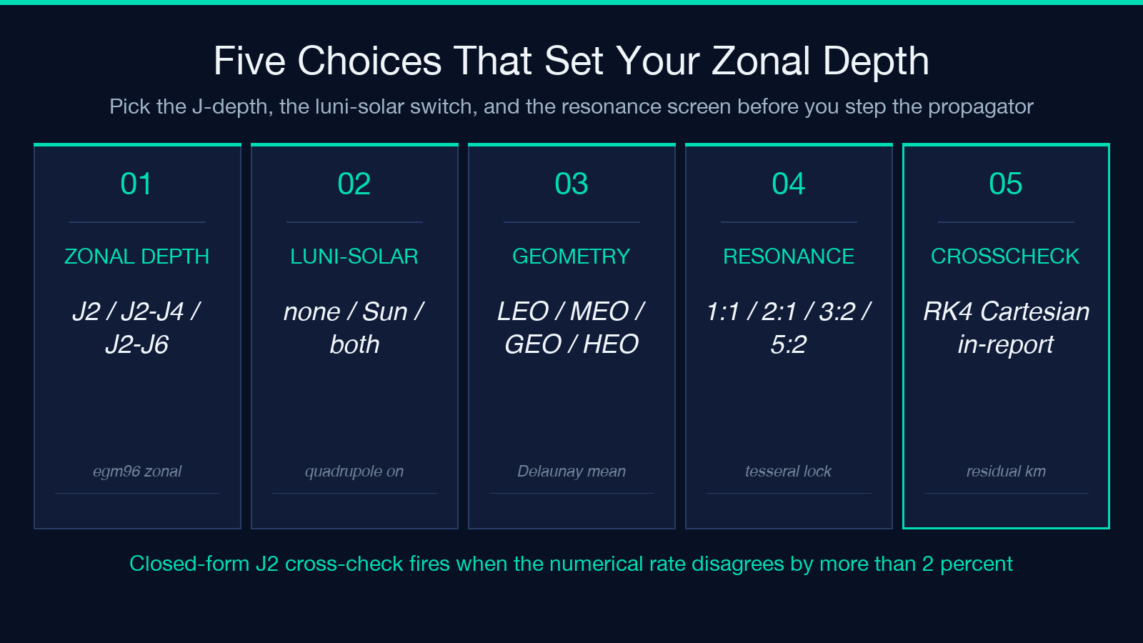
But if you propagate past two weeks without adding J4, the J4 contribution to Ω̇ shows up as an accumulating secular error. For a low-inclination LEO, J4 partially cancels J2 in Ω̇, and ignoring it produces a 0.4–0.8°/day drift over a month. The propagator’s J2–J4 mode keeps the J4 zonal harmonic in the orbit-averaged rate, which cuts that drift by an order of magnitude. J2–J6 is only worth the cost for high-inclination LEO (i > 70°), where the higher zonal terms couple into perigee precession through the cos⁴i and cos⁶i factors. For a 52.5° LEO, J2–J4 is the right depth; for a 98.6° sun-synchronous orbit, J2–J6 is justified.
A useful diagnostic the tool exposes is the closed-form cross-check: it prints the analytical J2 rate alongside the numerically-averaged rate, and flags disagreement above a configurable threshold. For most geometries the two agree to better than 0.5% — when they don’t, you are looking at a case where the numerical averaging has drifted off the canonical Delaunay normalisation, and the right move is to drop to J2-only and inspect the geometry before adding harmonics back.
The Luni-Solar Switch Is Not Free
Double-averaged luni-solar quadrupole is the term that drives the famous GEO inclination growth of roughly 0.75–0.95°/year. If you care about station-keeping north/south, you cannot leave it out. If you are propagating a LEO for a month, leaving it in costs you almost nothing in accuracy and adds the Kozai–Lidov critical mutual inclination diagnostic, which sits at arccos(√(3/5)) = 39.23° for the double-averaged quadrupole. For a satellite in equatorial LEO, the Sun and Moon are far enough from the critical inclination that the term is essentially a secular drift in Ω and i. For a satellite in HEO above 25,000 km with moderate inclination, the term is the dominant non-zonal perturbation and the propagator’s RK4 cross-check tells you in seconds whether your averaged model is still the right tool.
The diagnostic the tool surfaces is a small panel that prints the luni-solar contribution to each rate in degrees-per-day, plus a flag for whether the mutual inclination between the satellite orbit plane and the perturber orbit plane is within 1° of the Kozai–Lidov critical value. For most LEO and MEO geometries that flag stays off. When it lights up, you have a satellite whose long-term evolution is going to be dominated by the quadrupole, and you should consider whether the averaged model is valid at all — for very high-eccentricity orbits near the critical inclination, the Kozai–Lidov cycle mixes short-period and secular terms in a way that the orbit-averaged decomposition can no longer cleanly separate.
Mean → Osculating Is a Reconstruction, Not a State
The short-period J2 deviations between the mean and osculating elements can be reconstructed analytically to first order, and the propagator exposes this as a separate pass that adds the short-period terms back to the mean-element history to produce the osculating-element history. This is useful for two distinct workflows. The first is comparing against an external ephemeris that publishes osculating elements — you need to reconstruct from your mean elements before the comparison is meaningful. The second is generating a Cartesian state vector from mean elements for input to a downstream numerical integrator — you want the osculating state, not the mean state, because the mean state is not a physical state.
The reconstruction is first-order, so it is accurate to a few hundred metres at LEO and degrades as the orbit gets more eccentric or the J2 contribution gets larger. For LEO with e < 0.1, the reconstruction error is usually below the RK4 cross-validation residual. For LEO with e > 0.2, or for any HEO, the reconstruction error becomes the dominant term in the comparison against a high-fidelity numerical propagator. The tool exposes this as a separate residual chart, and the right way to read it is to compare the reconstructed osculating residuals against the RK4 Cartesian residuals — when the two diverge, the J2 short-period reconstruction is the bottleneck.
Tesseral Resonance and the Ground-Track Screen
The ground-track repeat period is one of those numbers that quietly breaks mission planning if it is wrong. A satellite that is supposed to fly a 233-revolution ground track every 46 days needs its nodal precession to match the Earth rotation exactly; if the inclination is off by 0.05°, the ground track drifts by a few kilometres per day and the revisit cadence is gone. The propagator’s tesseral resonance screen computes the ground-track repeat ratio as Ω̇/(360°/day − n) and classifies it into 1:1 (geosynchronous), 2:1 (semisynchronous), 3:2 (Molniya-class), 5:2, and a continuous band of small-rational commensurabilities. For each classification it prints whether the geometry is stable, marginally stable, or inside a resonance lock-in.
The Molniya 12-hour orbit is the canonical resonance case: the argument of perigee librates around 270° because of the J2–J4 coupling, and the ground track repeats every two revolutions. If your averaged model does not see the resonance, your perigee will drift instead of librate, and your apogee will migrate over months. The propagator handles this by computing the long-period J2–J4 coupling in ω̇ and flagging the libration regime. When the libration flag is on, the right move is to drop to a longer step and let the averaged model integrate through several libration cycles; when it is off, the secular model is fine.
The Three Diagnostic Passes That Decide Whether Your Geometry Is Right
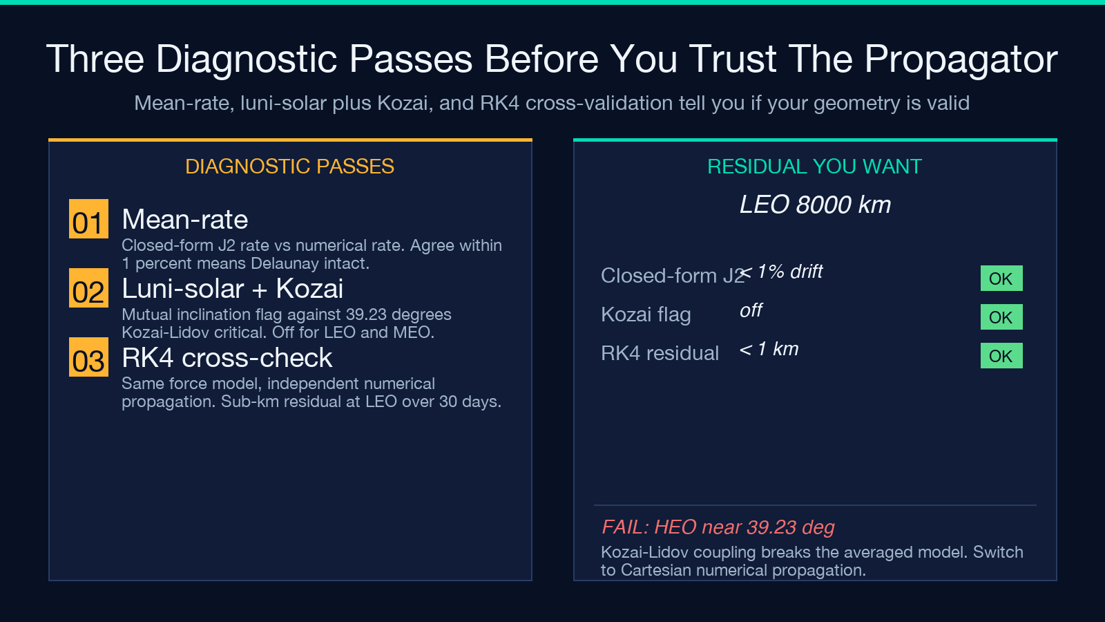
The propagator’s output is a single HTML report, but the report is organised so that three passes through it tell you everything you need to know about whether your geometry is valid for the averaged model:
1. Mean-rate pass. Print the closed-form J2 rate and the numerically-averaged rate for Ω̇ and ω̇. If they agree to better than 1%, the Delaunay normalisation is intact and your mean-element decomposition is valid. If they disagree by more than 5%, the geometry is outside the averaged model’s validity envelope and you need a Cartesian numerical propagator.
2. Luni-solar + Kozai pass. Print the luni-solar contribution to each rate and the Kozai–Lidov critical inclination flag. If the flag is on and the satellite is in HEO, the averaged model is going to drift over months. If the flag is off, the luni-solar term is a small secular correction and the averaged model is fine.
3. RK4 cross-validation pass. Run the report’s in-report RK4 Cartesian numerical propagation with the same force model and compare the residuals against the reconstructed osculating elements. The residuals should be sub-kilometre at LEO for a 30-day window, sub-decakilometre at MEO, and at the limit of the averaged model’s validity at GEO. When the residuals are larger than that, the bottleneck is the short-period J2 reconstruction, and the right fix is to either reduce the propagation window or accept that the averaged model is the wrong tool for the geometry.
Where the Averaged Model Breaks Down
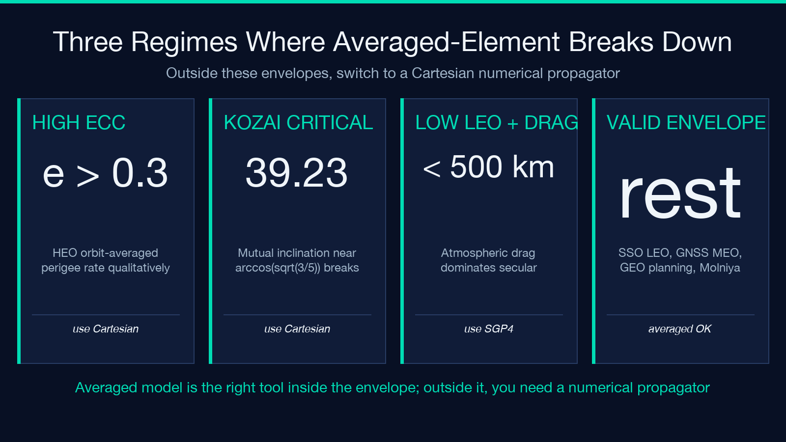
The averaged model is wrong in three regimes, and it is worth knowing them up front:
- Eccentricities above ~0.3. The Delaunay normalisation assumes small eccentricity. For HEO with e > 0.3, the orbit-averaged rate of
ω̇from J2 is qualitatively wrong, and the averaged model will diverge from a Cartesian propagator over weeks. - Inclinations inside 1° of the Kozai–Lidov critical mutual inclination. The double-averaged quadrupole approximation breaks down here because the short-period and secular terms couple. For a satellite in this regime, the averaged model needs to be replaced with a Cartesian numerical integrator.
- Low-altitude LEO with significant drag. The averaged model does not include atmospheric drag. For LEO below 500 km, drag dominates the evolution over weeks and the averaged model is the wrong tool.
For everything else — sun-synchronous LEO, GNSS MEO, GEO station-keeping planning, Molniya and Tundra HEO outside the Kozai–Lidov critical regime — the averaged model is the right choice, and the propagator gives you the diagnostic passes that let you confirm it in seconds rather than days.
A Worked Example: 30 Days of LEO Propagation
A practical baseline is a LEO at 8000 km semi-major axis (about 1637 km altitude), eccentricity 0.05, inclination 52.5°, propagated for 30 days at J2–J4 depth with no luni-solar term. The report should show RAAN drifting at about −2.76°/day and perigee at about +1.9°/day, both within 2% of the closed-form J2 rates. Eccentricity and inclination should be stable to better than 10⁻⁵ over the window. The ground-track repeat ratio should come out at about 12.13 revolutions per day, which is a small-rational commensurability that the tesseral resonance screen will flag as a stable ground track. The RK4 numerical cross-validation should show a sub-kilometre residual against the reconstructed osculating elements at the end of the 30-day window. When all three of those checks pass, your geometry is in the averaged model’s validity envelope, and you can propagate with confidence.
If you want to extend that same baseline to a year, drop the luni-solar switch off (it is negligible at LEO), keep J2–J4, and re-run. The inclination should drift by less than 0.01°/year from the secular J2 effect. The ground-track repeat ratio will hold to the fourth decimal. And the RK4 cross-validation residual will still be sub-kilometre at the end of the year, which is the diagnostic that says the averaged model is the right tool for this geometry.
The Take-Away
Averaged-element propagation is a workflow, not an algorithm. The algorithm is the orbit-averaged Gauss variational rates; the workflow is picking the right J-depth, deciding whether the luni-solar term is significant, running the closed-form J2 cross-check, screening for Kozai–Lidov critical inclination, classifying the ground-track resonance, and validating against an in-report RK4 numerical propagation with the same force model. The tool packages all six steps into one HTML report. Run the Brouwer–Lyddane propagator on your geometry, walk the three diagnostic passes, and you will know within a few seconds whether the averaged model is the right tool for the job — or whether your geometry is one of the three regimes where you need to step up to a Cartesian numerical integrator.
For more online tools, browse the full Elysia Tools catalogue.
