

A negative radicand is the Bernoulli solver telling you the flow cannot exist. Plug in v₁ = 4 m/s, p₁ = 200 kPa, z₁ = 10 m and a downstream pressure of 320 kPa with the same elevation, and the tool refuses the velocity solve because v₂ would have to be imaginary. The Bernoulli equation has no fudge factor for that case — it just returns an error and a labeled reason. That refusal is the most useful answer the tool ever gives, because it surfaces upstream/downstream pairing mistakes before any pipe is welded.
The Bernoulli equation solver takes the upstream triplet (pressure, velocity, elevation) plus any two of the three downstream quantities, then solves the third from p/(ρg) + v²/(2g) + z = const. Density and gravity are accepted in mixed SI / metric / imperial units; the result is returned as a labeled JSON object with the upstream and downstream heads plus the total head, so the same input feeds both an audit trail and a back-of-envelope check.
Why the Bernoulli equation is still the right starting point for ideal flow
The Bernoulli equation is the energy-conservation statement for steady, ideal, incompressible flow along a streamline. It says the sum of pressure head p/(ρg), velocity head v²/(2g), and elevation head z does not move as you walk along the streamline — only its components trade against each other. Most fluid-mechanics tooling offers the full Navier–Stokes equation by default, which is the right call for viscous, compressible, or unsteady flow. For a venturi meter, a tank drain, a Pitot probe, or any pipe section where the Reynolds number is high and the Mach number is low, the Bernoulli equation is exact enough to drive the design and short enough to drive the audit.
The Bernoulli equation solver exposes each of those three heads as a labeled field, plus the total head and the chosen unit set. Upstream pressure, velocity, and elevation appear alongside their head equivalents so any unit mistake (a pressure still in bar when the rest are in Pa, an elevation still in feet when the rest are in metres) becomes obvious in the JSON output before any downstream quantity is computed.
Reading the four reported heads without confusion
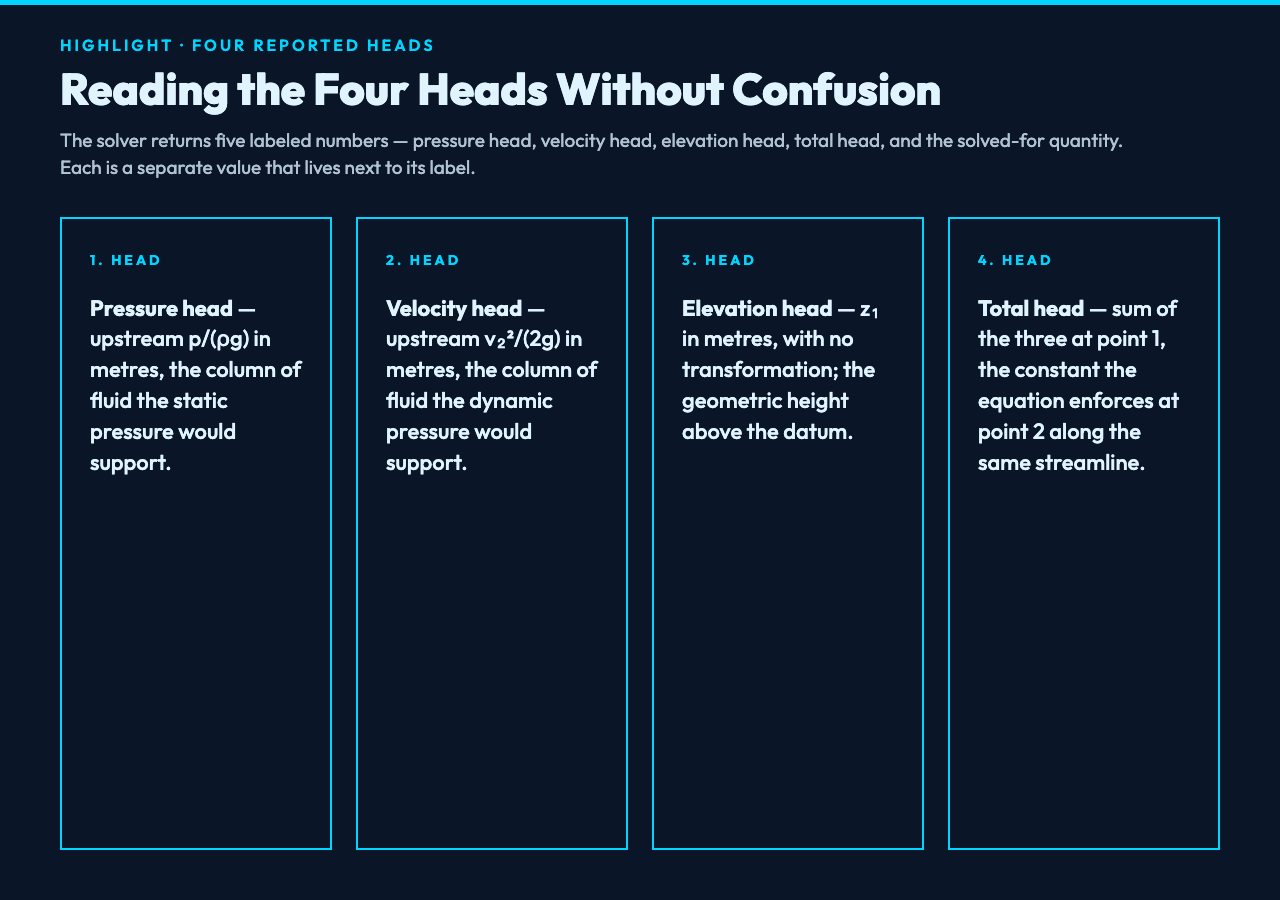
The calculator returns five labeled numbers. Pressure head is in metres, the upstream p/(ρg) term at point 1. Velocity head is in metres, the upstream v₂²/(2g) term at point 1. Elevation head is in metres, the elevation z₁ at point 1, with no transformation. Total head is in metres, the sum of the three at point 1, and is the constant the equation enforces at point 2. Solve output is the solved-for downstream quantity in its native unit (Pa for pressure, m/s for velocity, m for elevation) plus the head form of that same quantity.
A clean run with ρ = 1000 kg/m³, p₁ = 200000 Pa, v₁ = 4 m/s, z₁ = 10 m, and a downstream p₂ = 150000 Pa at z₂ = 10 m returns v₂ = √[16 + 2(50000)/1000] = √(16 + 100) = √116 ≈ 10.770 m/s. Velocity head jumps from 0.815 m to 5.913 m, pressure head falls from 20.387 m to 15.290 m, and the total head holds at 26.202 m within rounding. The math is exact; the auditing is in noticing which head your datasheet actually quoted.
Three failure modes the solver surfaces immediately
The Bernoulli equation is unforgiving in three specific ways that show up in real engineering checks. The first is the negative radicand on the velocity solve. The second is a density picked for the wrong phase. The third is an elevation that should have been a pressure head, or vice versa.
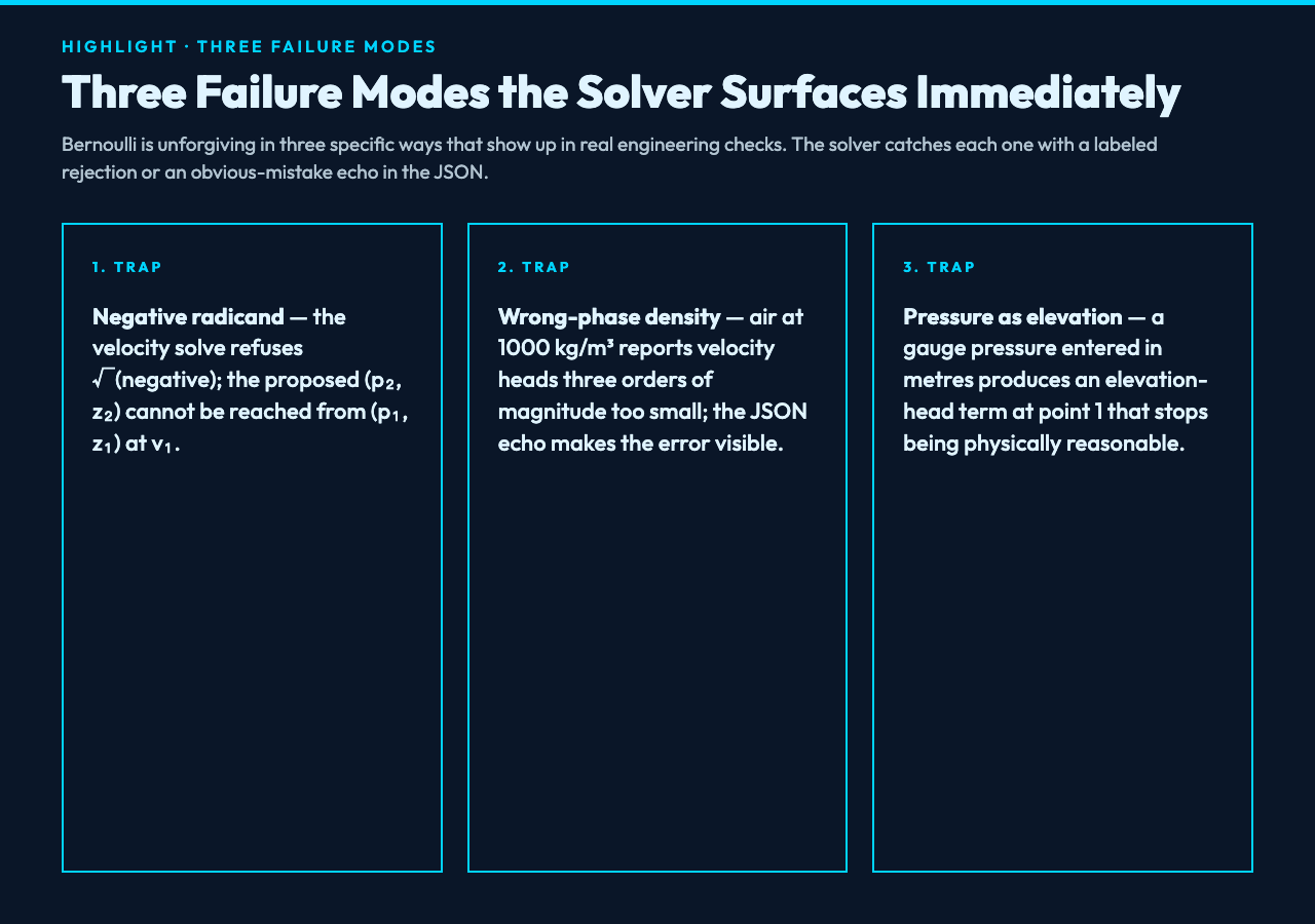
- Negative radicand on the velocity solve. A velocity solve returns v₂ = √[v₁² + 2(p₁-p₂)/ρ + 2g(z₁-z₂)]. When the bracketed term is negative, the square root is not real and the solve fails. Physically, the proposed (p₂, z₂) pairing cannot be reached from (p₁, z₁) at v₁ — the upstream pressure cannot push the fluid past a downstream pressure that high. The solver labels this as a negative radicand error so the audit trail is explicit.
- Density picked for the wrong phase. Air at 20 °C is about 1.204 kg/m³; water at 20 °C is 998 kg/m³. A venturi on an air line with ρ = 1000 kg/m³ reports velocity heads that are three orders of magnitude too small. The solver does not check phase, but the resulting pressure head at p = 200000 Pa becomes 0.020 m instead of 16.92 m — obviously wrong, and the JSON echo makes it visible.
- Elevation entered as a pressure head. The most common mistake is feeding a gauge pressure at the bottom of a tank as if it were an elevation in metres. The two have different units and the resulting total head is off by a factor that depends on ρg. The solver’s labeled head outputs flag this immediately because the elevation head term at point 1 stops being physically reasonable.
Five examples the solver handles cleanly
The tool accepts any combination of upstream (p, v, z) plus any two of (p₂, v₂, z₂), and reports the third. The five cases below cover the bulk of the engineering questions the model is asked.
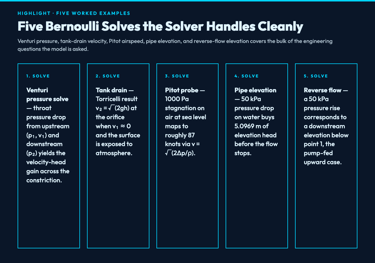
- Venturi pressure solve. ρ = 1000 kg/m³, p₁ = 200000 Pa, v₁ = 4 m/s, z₁ = z₂ = 0 m, v₂ = 10 m/s. Solve returns p₂ = p₁ + 0.5*1000*(16-100) = 142000 Pa. The pressure drop across the throat is what a venturi meter reads.
- Tank drain velocity solve. ρ = 1000 kg/m³, p₁ = p₂ = 101325 Pa, z₁ = 10 m, z₂ = 0 m, v₁ ≈ 0. Solve returns v₂ = √(0 + 0 + 2*9.81*10) = √(196.2) ≈ 14.007 m/s. The classic Torricelli result.
- Pitot probe airspeed solve. ρ = 1.204 kg/m³, p₁ = 101325 Pa, v₁ ≈ 0, z₁ = z₂, p₂ = 102325 Pa. Solve returns v₂ = √[0 + 2(1000)/1.204 + 0] = √1661 ≈ 40.76 m/s. The 1000 Pa stagnation pressure corresponds to roughly 87 knots at sea level.
- Pipe elevation solve. ρ = 1000 kg/m³, p₁ = 250000 Pa, v₁ = 2 m/s, z₁ = 0 m, p₂ = 200000 Pa, v₂ = 2 m/s. Solve returns z₂ = z₁ + (p₁-p₂)/(ρg) + (v₁²-v₂²)/(2g) = 0 + 50000/(1000*9.81) + 0 = 5.0969 m. The 50 kPa pressure drop buys 5.1 m of elevation head, which is the height a downstream tank can sit before the flow stops.
- Reverse-flow elevation solve. Same as case 4 with p₂ = 300000 Pa instead of 200000 Pa. Solve returns z₂ = 0 – 50000/(1000*9.81) + 0 = -5.0969 m. The pressure rise at point 2 corresponds to a downstream elevation below point 1, which is the configuration of a pump-fed upward line.
Why the streamline assumption quietly limits the model
Bernoulli holds along a streamline, not across streamlines. The solver does not check whether the two points are on the same streamline — it assumes they are. For a straight pipe at constant cross-section, that assumption is exact. For a pipe with a branch, for a tank with a swirl, or for any flow with significant transverse motion, the two points may be on different streamlines and the equation no longer holds. The solver returns the right answer for the wrong question; the engineer has to know whether the geometry qualifies.
When the Bernoulli equation is the wrong tool
Bernoulli assumes steady, ideal, incompressible flow. Three classes of problem break that assumption and need a different model.
- Compressible flow above Mach 0.3. The constant-density assumption fails; use a compressible-flow tool that handles the stagnation enthalpy form.
- Viscous flow with significant friction loss. Long pipelines, small-diameter tubes, and high-viscosity fluids need a Darcy–Weisbach or Hazen–Williams head-loss correction. Bernoulli returns the no-loss answer; the actual head at point 2 is lower by the friction term.
- Unsteady or pulsating flow. A water-hammer event, a positive-displacement pump pulse, or any time-varying inlet needs the unsteady Bernoulli equation with an added ∂v/∂t term. The steady solver assumes ∂v/∂t = 0.
How the solver handles unit and sign conventions
Density is accepted in kg/m³ or g/cm³; the solver converts internally. Pressure is accepted in Pa, kPa, bar, atm, or psi. Velocity is in m/s. Elevation is in m, cm, or ft. Gravity defaults to g = 9.81 m/s². All input quantities may be positive or negative within physically reasonable bounds, and the solver returns the sign of the solved-for quantity in the same convention. The JSON output carries every intermediate so the result is auditable step-by-step — no hidden constants, no silent conversions.
The Bernoulli equation solver is the right tool for any streamline problem where ideal flow is a fair assumption, and the wrong tool for the rest. For a broader view of how Bernoulli fits alongside other fluid-mechanics calculators, browse the full elysia-tools catalog and look for the Math & Numbers cluster.
Verifying a textbook Bernoulli problem against the solver
The standard audit pattern is: take a worked example from a textbook chapter on ideal flow, convert all values to Pa, m/s, m, kg/m³, run them through the solver, and check whether the solved-for quantity matches the textbook’s answer within rounding. If it does, the unit handling matches the textbook’s convention. If it does not, one of the four inputs is in the wrong unit — usually the elevation, because feet and metres are the easiest to mix up when the rest of the problem is in SI. The solver makes the audit a few-keystroke operation, and the JSON output becomes the receipt you attach to the back-of-envelope check.
The same audit loop catches the most common engineering mistake in ideal-flow work: a Bernoulli calculation that “looks right” by total head but fails a measurement because the streamline assumption does not hold. The Bernoulli equation solver surfaces the assumption failure indirectly, by returning physically reasonable answers for the wrong geometry, and directly, by refusing a negative radicand on the velocity branch.
