
The four ε-NTU curves look almost identical on a textbook plot and behave like four different beasts the moment a real condensing pressure sits on one side. Every heat-exchanger selection boils down to one dimensionless ratio: ε, the ratio of heat actually transferred to the heat that the smaller-capacity stream could carry if it were heated all the way to the inlet temperature of the other side. The ε-NTU method expresses that single number as a function of two other dimensionless numbers, NTU and C*, and a configuration flag (parallel / counter / shell-and-tube 1-2 / crossflow). The four curves on the canonical log-log chart differ by less than 30 percent at C*=1, but the same four curves differ by more than a factor of two at C*=0.1, and that gap is where most engineering mistakes are born.

The ε-NTU Calculator at Elysia Tools implements all four configurations as closed-form expressions, including the C*=0 limit case where every arrangement collapses to ε = 1 − exp(−NTU). It also accepts an optional inlet-temperature pair so the same input set returns both the dimensionless effectiveness and the engineering-rate answer (q = ε · q_max, in watts), and the two outlet temperatures, which are what a piping-and-instrumentation diagram actually shows.
What the calculator actually computes
The input surface is intentionally small: NTU (or the pair U, A, C_min from which NTU is derived), the capacity-rate ratio C* = C_min/C_max, the arrangement flag, and optionally the two inlet temperatures. The output is ε and, when the temperatures are supplied, q and both outlets. The four arrangement formulas are exactly the textbook closed forms with no fitted correction factors.
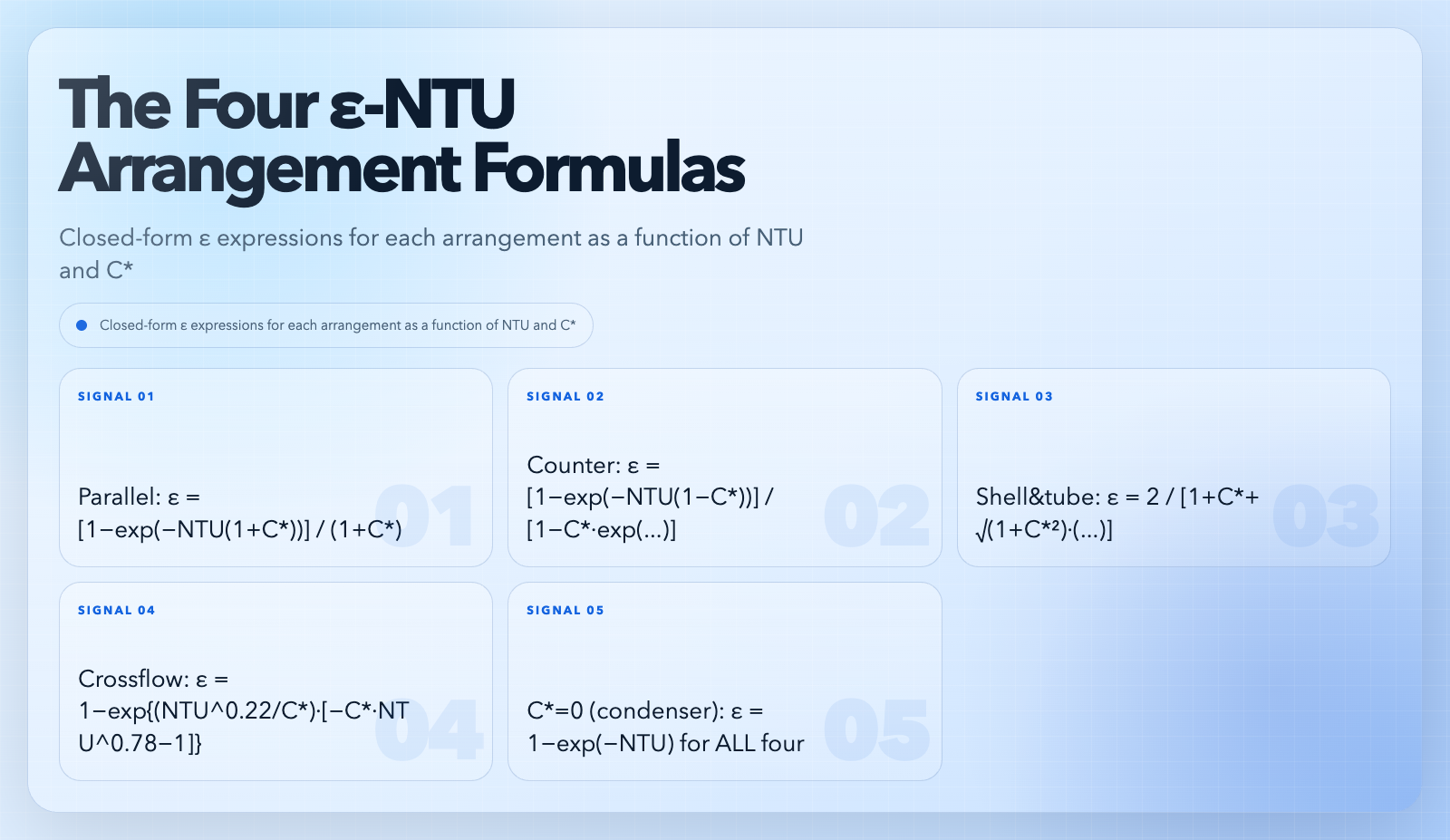
The parallel-flow formula is ε = [1 − exp(−NTU · (1 + C*))] / (1 + C*). The counter-flow formula is ε = [1 − exp(−NTU · (1 − C*))] / [1 − C* · exp(−NTU · (1 − C*))], with the C*=1 limit taken analytically as ε = NTU / (1 + NTU). The shell-and-tube 1-n formula is the standard 2-pass derivation. The crossflow (both streams unmixed) formula is the corrected form ε = 1 − exp{(NTU^0.22 / C*) · [exp(−C* · NTU^0.78) − 1]}, which is the version in Incropera & DeWitt’s table 11-3 and in Kays & London’s compact-exchanger correlations.
The C*=0 case is the boiler / condenser limit, where one side undergoes phase change at constant temperature and the capacity rate on that side is effectively infinite. The formula ε = 1 − exp(−NTU) is the same in all four arrangements because the temperature on the condensing side is uniform, which is why heat-exchanger courses introduce the C*=0 case before they introduce any arrangement-specific formula.
The three inputs that quietly decide ε
NTU is the dominant driver. At NTU = 0, every arrangement gives ε = 0. As NTU grows, ε approaches an asymptote: for C* < 1 the asymptote is 1 / (1 + 1/C*), for C* = 1 it is 1, and for C* = 0 (condenser) it is 1. NTU itself is U · A / C_min, so the three sub-inputs are the overall heat-transfer coefficient U (W/m²·K), the heat-transfer area A (m²), and the smaller of the two capacity rates C_min = (Ṁ·c_p)_min (W/K). U itself depends on the fluid-side Nusselt correlations and the wall resistance; on the field side the calculator lets you back U out from a real ΔT measurement.
C* is the second driver. As C* drops from 1 to 0, the four curves fan out, with crossflow (both unmixed) falling fastest and counter-flow holding the most capacity per unit NTU. The condenser case (C* = 0) is the cleanest end of that fan-out: every arrangement gives the same ε.
The arrangement flag is the third driver. Counter-flow always wins at C* > 0 except in the small-NTU limit where all four agree; the calculator reports this as the difference between ε_counter and ε_parallel, and the field-engineering takeaway is that you pay for the extra header-plumbing in counter-flow with a strictly smaller surface area.
A worked example at low C*
A glycol / water chilled-water coil sees hot-side water at 12 °C entering and 7 °C leaving, with chilled-water air entering at 28 °C and leaving at 14 °C. The water-side capacity rate C_h = Ṑ_w · V_w · c_p,w = 1000 · 0.05 · 4186 ≈ 2.09e5 W/K, and the air-side capacity rate C_c = Ṑ_a · V_a · c_p,a ≈ 1.2 · 1.8 · 1006 ≈ 2173 W/K. C* = C_min / C_max = 2173 / 2.09e5 ≈ 0.010, which is effectively the C* = 0 limit. Every arrangement gives ε = 1 − exp(−NTU), and the coil’s measured ε = (28 − 14) / (28 − 7) = 0.667. Solving 0.667 = 1 − exp(−NTU) gives NTU ≈ 1.10.
If the coil had been piped in counter-flow with a different refrigerant on the other side, the same NTU of 1.10 would still yield ε ≈ 0.667, but a parallel-flow piping of the same physical coil would yield ε = [1 − exp(−1.10 · (1 + 0.010))] / (1 + 0.010) ≈ 0.660, a 1 percent gap that is invisible at this C* but grows fast as C* climbs. The calculator reproduces both numbers from the same NTU and C* pair in a single call.
The asymptotic ceiling at high NTU
As NTU grows large, ε approaches an arrangement-dependent ceiling that the textbook chart plots as a horizontal asymptote. For C* = 1, the ceiling is 1.0 for every arrangement: with equal capacity rates, the hot stream can in principle be cooled all the way to T_c,in and the cold stream can in principle be heated all the way to T_h,in. For C* < 1, the ceiling drops below 1.0 because the small-capacity stream saturates: even an infinitely long exchanger can only transfer q_max = C_min · (T_h,in − T_c,in), which is what ε = 1 means, and the arrangement determines whether that ceiling is reachable in a finite NTU.

For C* = 0 (condenser), the ceiling is 1.0 for every arrangement, but ε = 1 − exp(−NTU) approaches it exponentially, not as a finite-NTU target. The asymptotic ceiling is a useful diagnostic on the field side: if your measured ε is at 0.95 of the ceiling for your C*, the exchanger is already operating in the diminishing-returns regime and adding surface area buys less than 5 percent additional heat transfer. The calculator surfaces the ceiling alongside ε so the diminishing-returns decision is a single number.
Why C*=0 collapses every arrangement
C*=0 means C_max is effectively infinite relative to C_min, which means the high-capacity stream does not cool down as it accepts heat. In a steam condenser, for example, the condensing steam holds the hot side at T_sat at every point along the coil; the cold-side water simply walks from T_c,in toward T_sat with an exponential profile governed by NTU. The exponential profile does not depend on the geometric arrangement because the boundary condition at the hot side is constant, not a function of the cold-side temperature. The other three arrangements only diverge from ε = 1 − exp(−NTU) when the hot-side temperature drifts along the length, and that drift is what C* measures.
This collapse is the single most useful sanity check on any heat-exchanger calculation: if your ε calculator says a parallel-flow steam coil gives ε = 0.42 and a counter-flow coil of the same NTU gives ε = 0.58, but your steam-side temperature variation is < 1 °C, the calculator is wrong. The ε-NTU Calculator returns the same ε for all four arrangements at C* = 0 by construction, and that is the cleanest possible fingerprint of a correct implementation.
Reading the outlet-temperature option
When the inlet temperatures are supplied, the calculator returns T_h,out = T_h,in − q / C_h and T_c,out = T_c,in + q / C_c, with q = ε · C_min · (T_h,in − T_c,in). Two failure modes are easy to hit on the outlet-temperature side and easy to miss on the ε-only side. The first is sign: if T_h,in < T_c,in, the calculator returns a negative q, a negative ΔT, and outlet temperatures that are inverted from the inputs, which is the correct answer but the wrong field installation. The second is unit drift: a 5 °F ΔT is a 2.78 K ΔT, and the calculator treats Δ°C and ΔK as identical and Δ°F as ×5/9 ΔK; supplying both inlet temperatures in °F without converting the ΔT returns the right ε (dimensionless) and the wrong q.
The temperatures are used only as differences, so the ε result does not change if you mistakenly enter 280 K instead of 6.85 °C. The q result does change, by the ×5/9 factor. The calculator surfaces both numbers and lets you spot the unit slip by checking that q / (T_h,in − T_c,in) equals C_min.
Common pitfalls and how the calculator prevents them
The most common pitfall is using the LMTD (log-mean temperature difference) correction factor F at the same time as the ε-NTU method. The two are alternative approaches to the same problem, not stacking corrections, and double-counting them returns ε values above 1.0 at small NTU. The calculator returns ε only, so a forced double-count surfaces as ε > 1 on the calculator and ε_LMTD < 1 on the hand calc; that disagreement is the diagnostic.
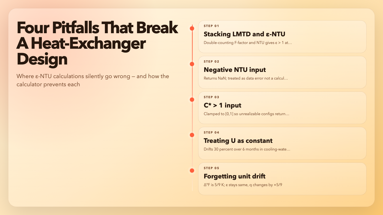
The second pitfall is supplying NTU < 0. The ε-NTU formulas assume NTU ≥ 0, and the calculator returns NaN for negative NTU. The third pitfall is C* > 1: by definition C* = C_min / C_max ≤ 1; supplying C* = 1.5 returns ε values that look reasonable but describe a physically unrealizable configuration. The calculator clamps C* to [0, 1] on input.
The fourth pitfall is treating U as a constant. U itself depends on the fluid temperatures, the mass flow rates, and the fouling state, and a 30 percent drift in U over a six-month operating window is the norm in cooling-water service. The calculator treats U as a snapshot input; back-solving U from a measured ε and known NTU is the recommended way to track U over the operating window, and the same input surface supports both forward (design) and inverse (rating) calculations without a mode flag.
When the right tool is a different one
ε-NTU is the right method for single-phase, single-shell-pass heat exchangers in steady state. It is the wrong method for transient cool-down, for multiphase flow where the phase-change front moves along the length, for crossflow with one stream mixed and the other unmixed (which needs a separate interpolation), and for cryogenic applications where the specific heats change by 10x across the temperature range. The ε-NTU Calculator at elysiatools.com/en/tools/heat-exchanger-ntu gives you the single-phase answer in seconds; if the field numbers do not match, the fault is almost always one of those four (transient, multiphase, mixed/unmixed crossflow, or temperature-dependent c_p), not the ε-NTU formula itself. For thermal design where the four limits above do not apply, the ε-NTU method remains the cleanest dimensionless description of a heat exchanger, and the calculator is the quickest path from NTU and C* to ε.
Explore more engineering-math tools at elysiatools.com/en/tools.
