Convolution Integral Field Guide: When the Formula Is Right and the Window Is Not

A convolution can be mathematically correct and numerically wrong at the same time. The integral (f*g)(t) carries no approximation of its own, and the tool that evaluates it uses a fourth-order quadrature rule that is already sitting at the float-precision floor for these integrands. Yet with the default window, the same tool that returns 3.6788 to five significant figures at t = 10 returns a value 20 percent too low at t = 25, and exactly half the true answer at t = 40. Nothing is broken. The upper bound on the integration window is doing it, silently, and the output never says so.

What the tool actually computes

The Convolution Integral Calculator on Elysia Tools takes two expressions, a mode, a window, and a list of output points. Write f(tau) and g(tau) in a single variable x, and the tool evaluates the integrand f(tau) * g(t - tau) at each of a set of quadrature nodes.

Two modes decide where the integral actually starts and stops.

In causal mode both signals are treated as zero for negative time, so the bounds become lo = max(tauMin, 0) and hi = min(tauMax, t). This is the Laplace-domain setup, the one you want for impulse responses and step responses.

In direct window mode the bounds stay exactly tauMin and tauMax, so the integral runs over the whole window regardless of t. This is the right choice for two-sided signals such as Gaussians, where truncating at t would cut off half the mass.

Underneath, the quadrature is the composite Simpson rule with an even number of subintervals, default 2000 and clamped to the range 100 through 20000. An odd count is bumped up by one, and the output header reports the adjusted count. The expressions themselves run through a shared allow-list evaluator: digits, letters, + - * / ^, parentheses and spaces, with a fixed set of functions (exp, sin, cos, tan, sqrt, ln, log10, and friends) and the constants e, pi and tau. Up to eight output points per run.

The bound that decides every number

Here is the whole story in two lines of arithmetic. In causal mode the upper bound is min(tauMax, t). The moment t exceeds tauMax, the upper bound stops following t and pins itself to the window edge, and from that point on the tool is no longer computing the convolution — it is computing the convolution with its tail removed.

That is not a numerical error. The quadrature is doing exactly what it was asked. The question that was asked is just smaller than the question you meant.

The same rule governs the lower bound in the other direction. lo = max(tauMin, 0) means a causal convolution genuinely does have zero output for negative time, so a row of zeros at t = -1 is correct rather than a failure.

The default window is tauMin = 0, tauMax = 20. Whether that default is generous or fatal depends entirely on how fast your signals decay.

The 20 percent error hiding behind a correct formula

Consider a pair of causal exponentials with a deliberately slow decay: exp(-x/10) convolved with itself. The exact causal convolution of two such signals has a closed form, t * exp(-t/10), so every claim below is checkable by hand.

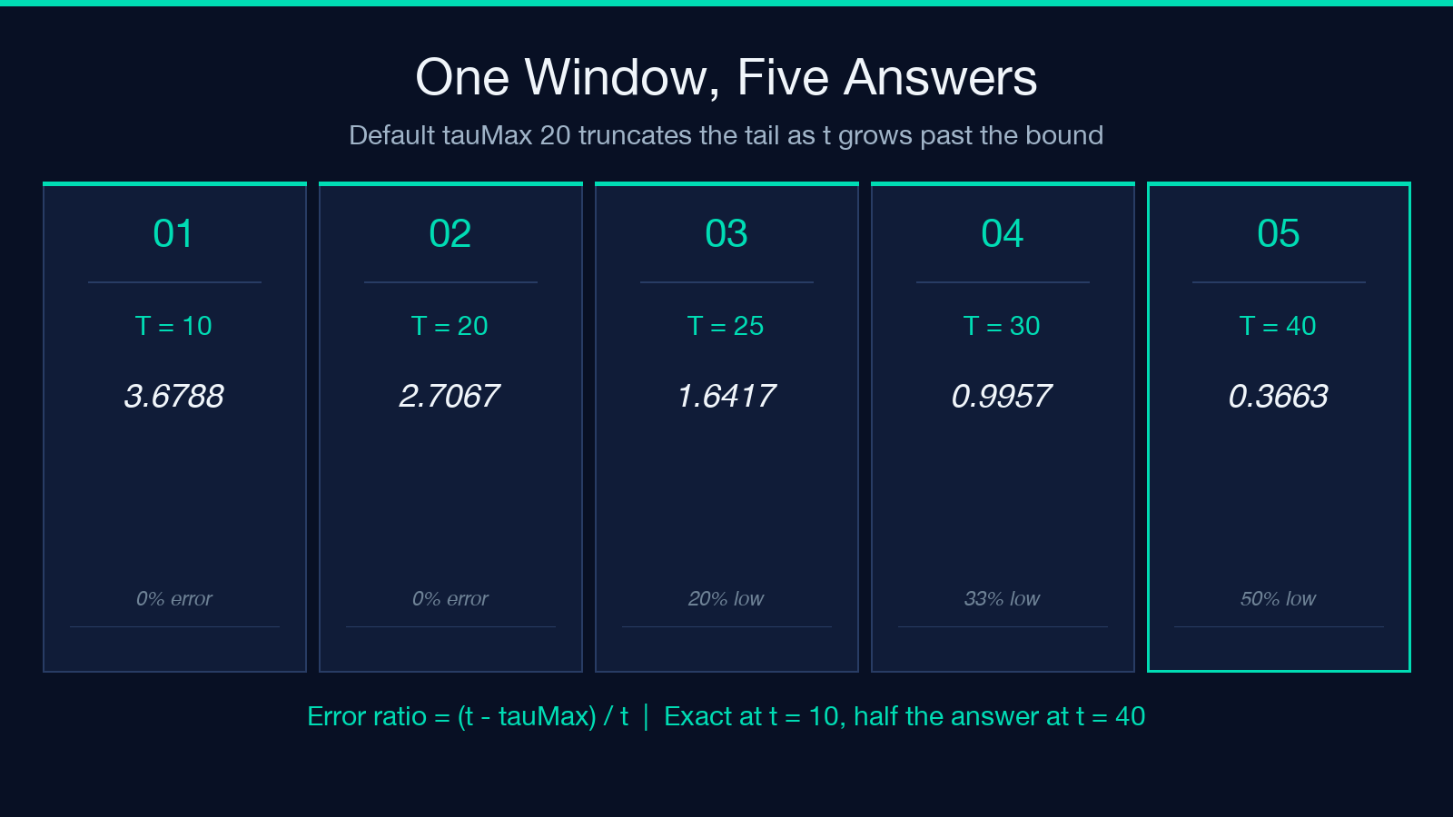
Run it with the default window [0, 20] and read off the tool’s output:

• t = 10 → tool reports 3.6788, exact value 3.678794, error 0.0 percent
• t = 20 → tool reports 2.7067, exact value 2.706706, error 0.0 percent
• t = 25 → tool reports 1.6417, exact value 2.052125, error 20.0 percent too low
• t = 30 → tool reports 0.9957, exact value 1.493612, error 33.3 percent too low
• t = 40 → tool reports 0.3663, exact value 0.732626, error 50.0 percent too low

Now the pattern, which is worth more than the individual numbers: the relative error is exactly (t - tauMax) / t, and it does not depend on the decay rate at all. At t = 25 the window clipped 5 units off a 25-unit interval, so it lost 5/25. At t = 40 it clipped 20 units off a 40-unit interval, so it lost exactly half. Change the decay constant from 10 to 50 and the error percentages do not move.

That is a much sharper diagnostic than “the number looks a bit low”. Once you know the error ratio, you can predict it before you run anything.

What Simpson’s rule fixes and what it cannot

The instinct after a bad answer is to raise the interval count. Measure it first. For the default exponential example at t = 1, the Simpson error scales as h to the fourth power — multiplying the error by n to the fourth gives a constant 0.001292 across n = 100, 200 and 400, exactly the fourth-order behaviour the rule promises.

But by n = 2000 the error has already fallen to 1.1e-16, which is the double-precision floor. Going to n = 8000 does not improve it; it wanders back up to 4.4e-16 as rounding noise starts to dominate. For a smooth integrand like this one, 2000 intervals is not a tuning knob. It is past the point where the quadrature matters at all.

So the error is never in the discretization. It is in the interval you asked it to integrate over, and no amount of subdivisions recovers a truncated tail. If you want to test whether a number is wrong, change tauMax and see if it moves. If it moves, you were window-limited, not resolution-limited.

Two windows, one expression

The fix is a single number, and it is worth watching the same expression produce two different answers.

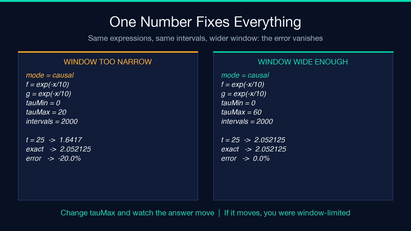
With tauMax = 20 the tool integrates exp(-x/10) against itself over [0, 20]. With tauMax = 60 it integrates over [0, 60], and because the causal upper bound min(tauMax, t) follows t all the way out, the answer becomes exact to float precision. Nothing else changed: same expressions, same mode, same 2000 intervals, same decimal places.

This is the single most useful habit the tool can teach. Before trusting any convolution output, ask what the window cost you. If t was near or beyond tauMax, the answer is a lower bound on the true value, not the value.

The rule of thumb: set tauMax several times the slowest decay constant in your signals. For exp(-x/10) that means tauMax in the low hundreds, not 20.

When the output says zero

Two separate mechanisms produce a literal zero, and they mean different things.

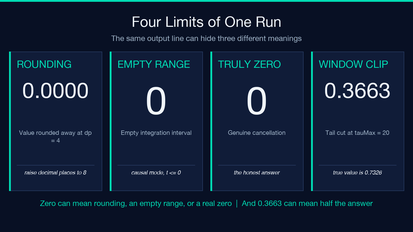
The first is display rounding. The tool rounds each value to a configurable number of decimal places, default 4, before printing it. The exact value at t = 10 for the default exp(-x) and exp(-2x) pair is 4.53979e-05. Rounded to four places that is 0.0000. So a row of zeros in the output usually means “the value fell below the display threshold”, not “the value is zero”. Raise the decimal places to 8 and watch the zeros become small numbers.

The second is an empty integration interval. When hi - lo is zero or negative the tool returns literal 0 without attempting the integral. In causal mode that happens for every t at or below zero, which is the correct answer for a causal signal, and it also happens if you set tauMin above your smallest t.

Both are visible in the output and neither is an error state. But a tool that reports 0 for “below the display threshold”, “before the signal starts” and “genuinely zero” with the same glyph is asking you to keep three different meanings in your head at once.

Reading the output honestly

Five rules cover the output of this tool, and each one corresponds to a specific line of the implementation rather than to general numerical advice.

• Window first. If t was near or beyond tauMax, the result is truncated. Widen the window before you widen anything else.
• Zero is ambiguous. Below the display threshold, before the interval starts, or genuinely zero — the glyph does not distinguish them.
• Intervals are not the lever. At 2000 subintervals the quadrature error is already at the float floor for smooth integrands.
• Odd counts get bumped. An odd interval count is rounded up to the next even number, and the header line shows the count actually used.
• Eight points is the cap. A ninth output point is rejected outright, so batch across runs rather than one long list.

The related Simpson’s Rule Integrator on Elysia Tools is the right companion when you want a single definite integral rather than a sliding one, and the Trapezoidal Rule Integrator is a useful cross-check: run the same integral both ways and watch the trapezoid rule’s error dwarf the window effect you were chasing. If you want the derivative of your convolution instead of the integral, the Numerical Differentiation Calculator covers the other half of the pair. For a related stiff-system problem, the Runge-Kutta RK4 Solver takes the same approach to a different integral.

Where to take it from here

The lesson is not really about convolutions. It is that a tool which is right about everything except one input can still be wrong in a way that looks like a bug in the mathematics. The Simpson rule is doing its job; the expressions are doing their job; the mode is doing its job. The one number that was not checked is the one that mattered, and no amount of precision in the other settings would have surfaced it.

The same discipline applies to every windowed numeric tool: before you trust a result, find the bound that decides it, and push that bound until the number stops moving. When it stops moving, the answer is real. When it keeps moving, you have found the actual question.

Browse the wider catalog at Elysia Tools for the rest of the math and numerics set.