
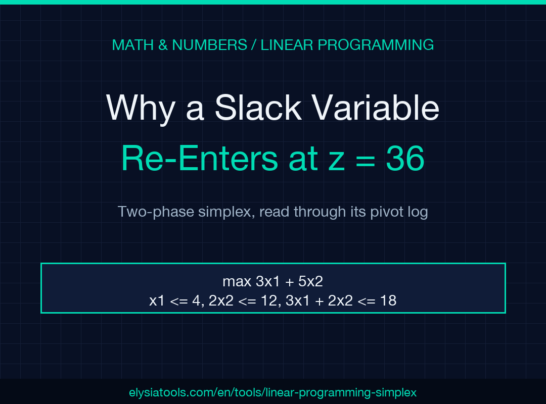
Three pivots carry the textbook product-mix problem to an objective of 36. The first two look sensible, but I keep rereading the third: the entering variable is s1, the slack of a constraint that went tight in pivot one, and x1 stays basic while its value drops from 4 to 2. The objective rises by 9 anyway. The simplex method does not climb toward better coordinates; it walks toward a better corner.
The third pivot lifts the objective while x1 falls
Walk the numbers. Maximize 3×1 + 5×2 subject to x1 <= 4, 2×2 <= 12, and 3×1 + 2×2 <= 18, with both variables nonnegative.
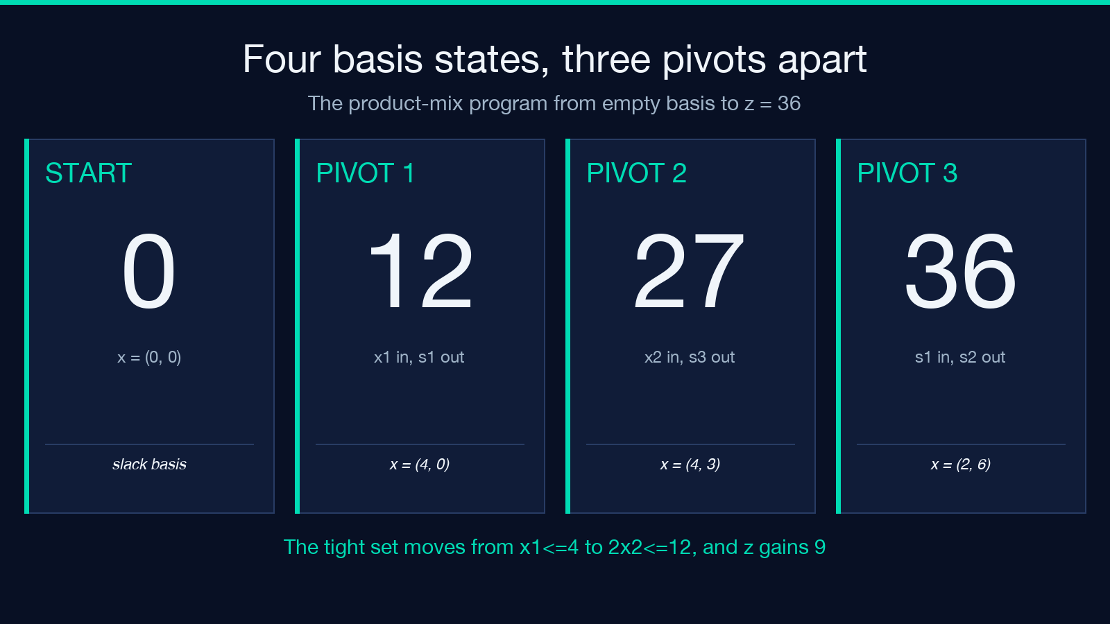
Pivot one brings x1 in and pushes s1 out: z = 12 at (4, 0). Pivot two brings x2 in and pushes s3 out: z = 27 at (4, 3). Both moves look like greedy improvement, and both pick the variable that pays more per unit of the resource that binds next. For example, pivot two raises the objective by 15, more than pivot one managed.
The third move refuses that story. s1 re-enters, s2 leaves, and the solution slides to (2, 6) for z = 36. The variable x1 stays basic, and its value falls by half while the objective gains 9.
What changed is the set of tight constraints. At (4, 3) the tight pair is x1 <= 4 and 3×1 + 2×2 <= 18. At (2, 6) it is 2×2 <= 12 and 3×1 + 2×2 <= 18. The first constraint now carries 2 units of unused capacity, and that capacity is the s1 column coming back. One row needs a second look: 3×1 + 2×2 <= 18 stays tight in both corners. A corner is a set of tight constraints, and the pivot that looks backward is the one that changes the set.
A tableau is bookkeeping, not a matrix you invert
The tableau never inverts anything. Each row is one constraint with its columns, and the basis records which column is basic in which row. In this case the basis holds exactly one column per row, and nothing else is stored.
Column layout follows one rule per row. A <= row gets a slack column of +1. A >= row gets a surplus column of -1 plus an artificial column. An = row gets an artificial column. The rightmost slot holds the right-hand side.
The decision rule is the reduced cost, z_j – c_j, and this engine takes the first column with a negative value in index order. Each iteration logs which variable entered, which left, and the objective after the pivot. That log is the data worth keeping. The answer is a byproduct.
Phase 0 rewrites the problem before any pivot runs
Negative right-hand sides break the starting basis, so the solver normalizes them first: multiply the row by -1 and flip the comparator. A <= row becomes >=, and >= becomes <=.
The rewrite is an identity, and the log proves it. I wrote min 2×1 + 3×2 subject to x1 + x2 >= 4 and x1 + 3×2 >= 6, then rewrote both rows with flipped signs and a negative right-hand side. Two phase-1 pivots, zero phase-2 pivots, x = (3, 1), z = 9 both times. Same path, same answer, measured twice on the same engine.
Phase 1 asks one question: can the artificials reach zero?
Artificial variables exist to give the first basis something to hold. They are fake columns with a penalty attached: phase 1 maximizes the negative sum of the artificials, so its objective starts below zero and climbs toward zero.
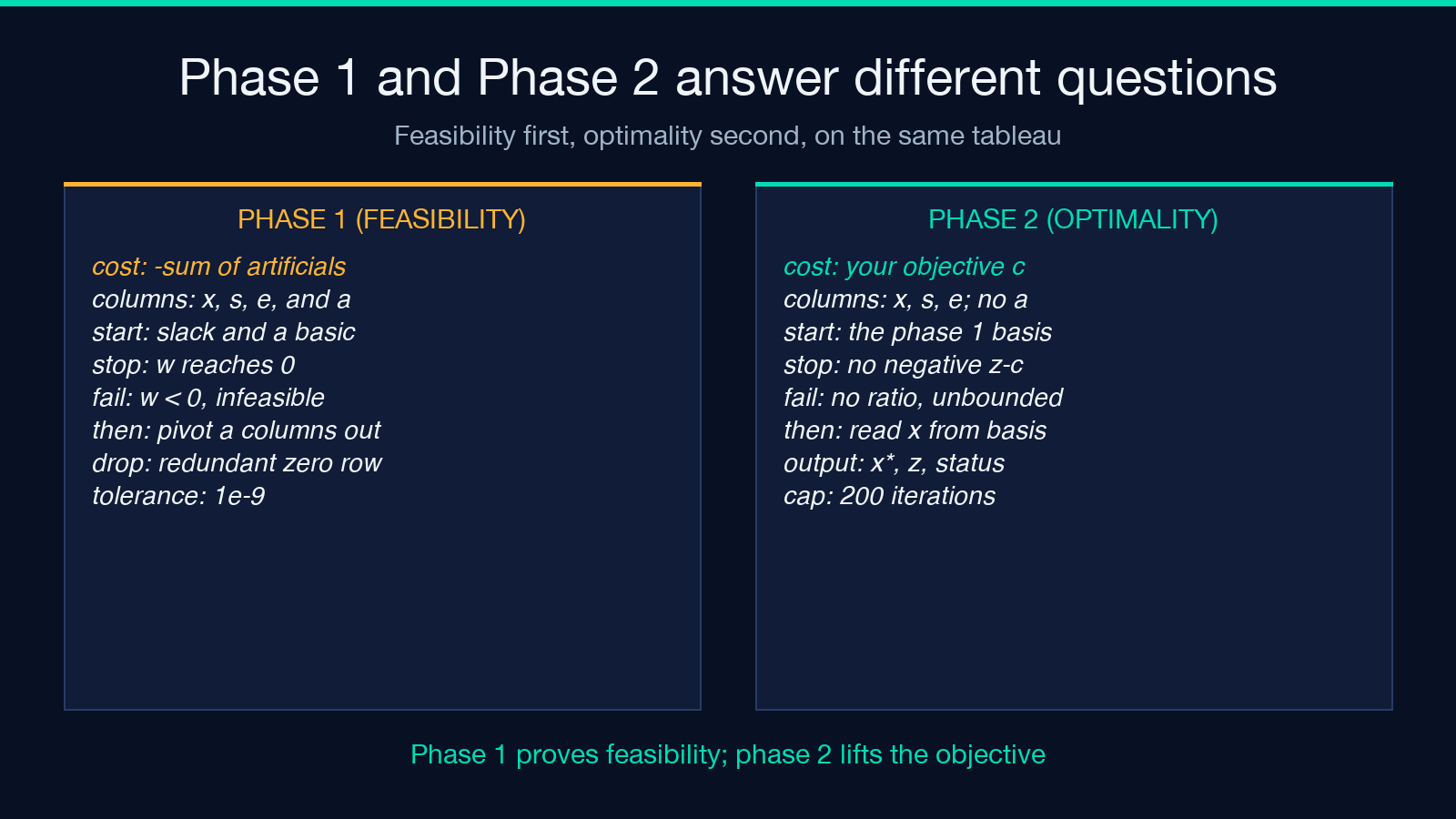
Zero means feasible. Anything left below zero means the original program has no solution, and the solver says so. Give it x1 + x2 <= 2 together with x1 + x2 >= 5 and phase 1 stops after one iteration with w = -3, then reports infeasible.
Once w reaches zero, remaining artificial basics get pivoted out, and a row with no other nonzero entry gets dropped as redundant. That is how an equality plus a slack constraint collapses into one row without an error. The log shows three objectives along that path: -2, then 0, then nothing left to fix.
Minimize is maximize with a sign at each end
The engine solves one problem: a maximization. A minimization is passed in with the objective coefficients negated, and the reported value is negated back.
The sign round-trip is cheap and worth watching. For min 2×1 + 3×2 the internal run maximizes -2×1 – 3×2, lands on (3, 1) with an internal value of -9, and the report flips it to z = 9. Both constraints hold with equality there, so the optimum sits on the intersection, not on an edge.
One detail from that run is more useful than the answer. The run I observed did zero phase-2 pivots. Phase 1 had already walked to the optimal vertex while chasing the artificials to zero, and the objective had nothing left to improve. Feasibility work can land on the answer.
Bland’s rule buys determinism, not speed
Ties are the failure mode of a naive simplex. When two rows give the same ratio, the choice decides whether the run terminates or cycles.
This solver uses Bland’s rule on both sides: the smallest index enters when several reduced costs are negative, and the smallest basis index leaves when ratios tie. The consequence is a hard guarantee of termination, since no basis repeats, plus a documented cap: 200 iterations as a backstop against numerical trouble at a tolerance of 1e-9.
The trade-off is real. Bland’s rule can traverse more vertices than the largest-improvement rule that commercial solvers use. What you buy is reproducibility: the same program produces the same pivot log on each run, which is what makes the log worth reading.
Infeasible and unbounded are proofs, not error messages
Neither status is a failure of the solver. Infeasible means phase 1 could not zero the artificials, so no point satisfies all the constraints at once. Unbounded means the entering column had no positive entry to ratio against, so the objective escapes to infinity along a ray.
The last line the engine writes is labelled “STATUS”, and it carries one of three words: OPTIMAL, UNBOUNDED, or INFEASIBLE. For instance, try max x1 + x2 subject to x1 – x2 <= 3. One pivot sets x1 = 3, then no row can limit x2, and the run stops with UNBOUNDED. All three statuses come with the iteration log that produced them, which is the part most tools omit.
Where this solver stops
The engine handles 2 to 6 variables and 1 to 8 constraints. That ceiling is deliberate: a tableau you can read by hand is a tableau you can learn from.
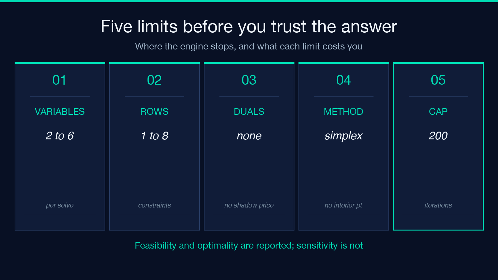
Two gaps matter if you plan to use it for real work. The report carries no dual values, according to its own output, so there are no shadow prices and no sensitivity ranges; the word duality shows up in the keyword list, not in the printed result. And there is no interior-point path, so a badly scaled 6-variable problem can still crawl.
Benchmark scale changes the calculus. HiGHS and Gurobi are built for thousands of rows and ship the warm starts this engine lacks. For the moment when you want to see why a pivot moved, open the two-phase simplex solver, paste the constraints, and read the log line by line. Explore more tools at elysiatools.com.
Two neighbours cover the steps around a solve, such as the second-order ODE solver for the dynamics a program might constrain and the residual calculator for checking a fit against measured values.
So the next time a solver hands you a per-iteration log, read the last pivot before you read the answer. Ask whether the constraint that went slack is the one you assumed was scarce, and whether the variable that fell is the one you were paying for. That is the question the log exists to answer, and it is the one a single number will never show you.
本文有中文版:松弛变量为何在 z = 36 时重回基变量
