
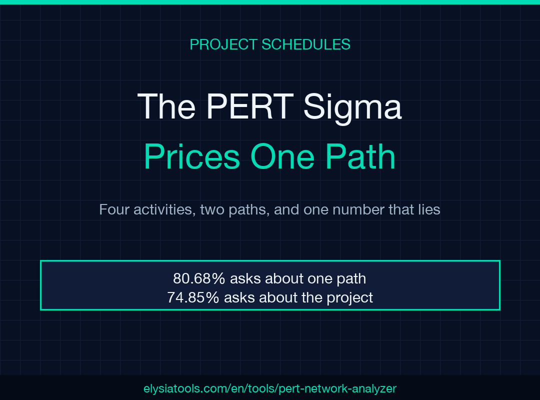
Four activities, three estimates each, one deadline. The PERT calculator returns an expected duration of 15 days and a standard deviation of 1.1547, feeds both into the normal curve, and reports an 80.68% chance of finishing by day 16. Keep the same four activities and the same twelve estimates, but count the second path as well, and the answer is 74.85%. Nothing about the estimates changed. Only the arithmetic wrapped around them did.
PERT prices the path you expect to win, then labels the result as the project.
That gap is not a rounding artifact, and it is not a bug in the calculator. It is the method working exactly as defined. Once you separate the two things PERT computes, an average per activity and a sum per path, the failure becomes easy to see and cheap to fix.
Three numbers per activity, two of them do the work
Each row of a PERT network carries an optimistic estimate a, a most likely m, and a pessimistic b. Two formulas consume them. The expected duration is te = (a + 4m + b) / 6, and the variance is σ² = ((b − a) / 6)².
The first is a weighted average with weights 1:4:1. The most likely value carries two thirds of the weight, so te mostly repeats what you already believed. The second formula does something different. It treats the whole range b − a as six standard deviations, three on each side of the mean, and squares the sixth of it.
The practical consequence is an asymmetry most estimators never notice. Take the activity A(2, 4, 6), with an expected duration of 4.0000 days and a variance of 0.4444. Now stretch the pessimistic estimate by two days, to A(2, 4, 8). The expected duration moves from 4.0000 to 4.3333, a third of a day, easy to wave through in a planning meeting. The variance moves from 0.4444 to 1.0000, an increase of 125%. A wider pessimistic estimate forces the variance up while barely moving the schedule.
So the number you defend hardest, m, sets the schedule. The number you barely discuss, the width of b, sets the risk. Teams spend the meeting arguing about m and then inherit a variance nobody designed or measured.
The classic network drops its own riskiest branch
Here is the textbook four-activity network, the one shipped as the tool’s own worked example. Four rows, four expected durations, one rejected column:
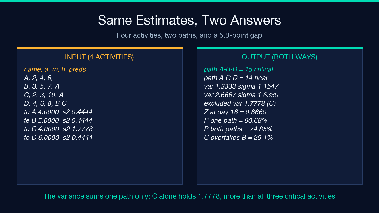
- A: optimistic 2, most likely 4, pessimistic 6 → te 4.0000, σ² 0.4444
- B: optimistic 3, most likely 5, pessimistic 7 → te 5.0000, σ² 0.4444
- C: optimistic 2, most likely 3, pessimistic 10 → te 4.0000, σ² 1.7778
- D: optimistic 4, most likely 6, pessimistic 8, after B and C → te 6.0000, σ² 0.4444
Two paths run from start to finish: A → B → D costs 4 + 5 + 6 = 15 expected days, and A → C → D costs 4 + 4 + 6 = 14. The critical path is A → B → D. The expected project duration is 15, and the project variance is the sum of the three variances on that path, 0.4444 + 0.4444 + 0.4444 = 1.3333, so σ = 1.1547.
Activity C contributed nothing to that sum. It sits on the 14-day path, one expected day short of the winner, so its variance was set aside. PERT cuts the variance budget at the critical path and discards the remainder. That discarded number is 1.7778, which on its own proves larger than the entire 1.3333 the tool kept for the whole project.
Read that again in plain terms. The single most uncertain activity in the network carries more variance than the three critical activities combined, and the reported project uncertainty excludes all of it.
The 14-day path wins one time in four
Dropping C would be defensible if the 14-day path could never finish last. It finishes last about a quarter of the time, a case the critical-path sum cannot represent.
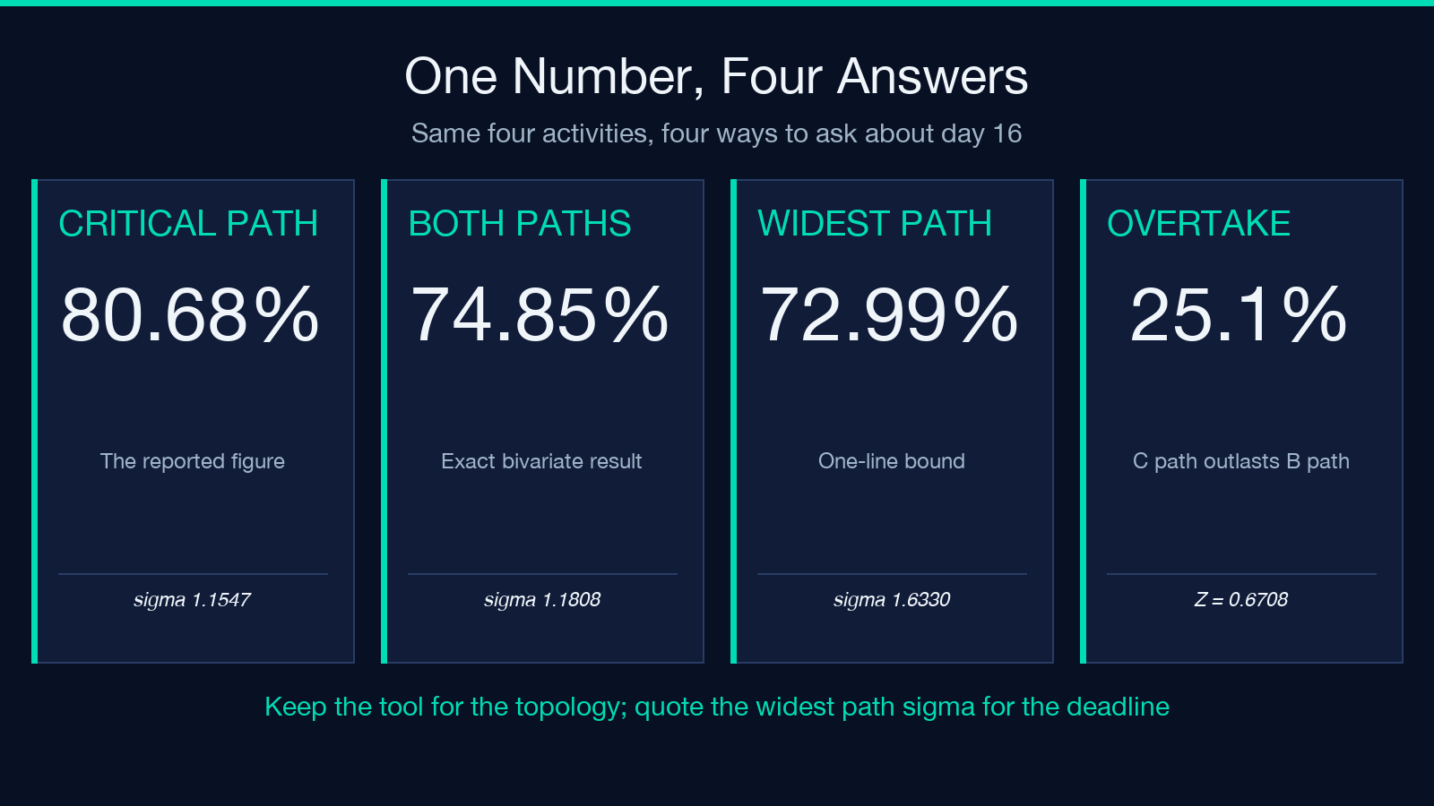
The two paths share activities A and D, so when one overtakes the other, the difference is only B versus C. B has mean 5 and variance 0.4444. C has mean 4 and variance 1.7778. The difference has mean 1 and variance 2.2222, giving a standard deviation of 1.4907 and Z = 0.6708. The probability that C’s path outlasts B’s is Φ(−0.6708) = 25.1%. One expected day creates all of that difference.
That is the merge bias, and in this case it moves the answer at the deadline. Keeping the tool’s own per-activity numbers and accounting only for the max of the two paths, the exact bivariate probability of finishing by day 16 is 74.85%, not 80.68%. An independent Monte Carlo over the same four normal distributions, with the same means and standard deviations, lands at 74.7% on 200,000 draws, which is sampling noise around the analytic value. Expected duration stays at 15.2272 days. The measured spread is 1.1808, not the 1.1547 the tool prints.
The assumption that a sum of means describes a maximum breaks here. Two paths in parallel do not average; the project takes whichever finishes later, and the maximum of two random variables is not the maximum of their means.
Take the variance formula itself. It is an assumption, not a derivation. For example, fit a standard beta shape to those same three points using the conventional PERT weights and the standard deviation comes out 13% wider than b − a over 6, because a beta with its mode at the midpoint is fatter than the ±3σ convention implies. Shape and path structure each add a slice of optimism, and they compound.
Point estimates turn a probability into a certainty
Set a, m, and b to the same value and the arithmetic collapses in a way that looks authoritative and means nothing. With a = m = b = 4, the expected duration is still 4 and the variance is exactly 0.
The tool is honest about it. When σ falls below 1e-9 it skips the normal curve and prints a deterministic line: sigma is zero because all estimates are point estimates, the project finishes exactly at the expected duration, and the completion probability is 1 if the target is at or beyond it, 0 otherwise.
So build a network from single-point estimates and it returns a 100% on-time probability against any deadline after the expected date. That is correct arithmetic over an empty uncertainty budget. It also means a neatly formatted “100%” can come out of a schedule whose inputs carry no risk data at all. If you see a probability of exactly 1 or exactly 0, check whether the inputs had any width before you treat the number as a forecast.
Two critical paths, one reported number
A network can have parallel critical paths. When it does, the text output lists them all, but the machine-readable summary reports a single path, the first one found. The probability is computed from the union of activities across each critical path. That union removes double counting when two critical paths share an activity, so the variance is a sum over distinct names, not over paths. The variance is not wrong. Only the named path is truncated.
This matters if anything downstream reads the structured output instead of the report. A dashboard, for instance, will show one chain while the variance quietly covers two or three. The text report and the metadata agree on the variance and disagree on the topology, and nothing in the interface clarifies the difference.
The input contract is stricter than the labels
The parser is unforgiving in ways the field labels do not advertise:
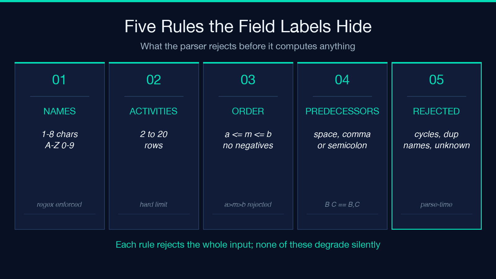
- Activity names must match a single alphanumeric token of one to eight characters. “Survey” works; “Site-Survey” and “Development” are rejected.
- A network needs at least two and at most twenty activities.
- Estimates must satisfy a ≤ m ≤ b, and the optimistic value cannot be negative, though zero is allowed, which is how you enter a milestone.
- Predecessors accept spaces, commas, or semicolons as separators, so “B C” and “B,C” are equivalent.
- Cycles, duplicate names, and predecessors that do not exist are rejected outright rather than silently ignored.
One display detail is worth knowing before you check the arithmetic by hand. The decimal-places setting rounds the printed te and variance columns, while the critical-path pass runs on the unrounded values. At one decimal place a printed column will not sum exactly to the printed expected duration. The totals are right. The columns are rounded.
Where the tool earns its keep
The parts of PERT that do not depend on the probability model are solid, and they are the reason to use a calculator instead of a spreadsheet formula. The forward and backward passes give early and late start and finish for each activity, slack is the gap between them, and the critical path is the set with zero slack. Ordering violations, cycles, and dangling predecessor references are caught at parse time, which is more than a hand-built model usually manages. The method dates from 1958, when the US Navy used it on the Polaris program, and the one-path variance convention has not moved since.
The same two passes let you compare estimate sets honestly. Feed in your current numbers, then feed in the version where the vendor slips a week, and read the change in expected duration and in variance separately. A better estimate of m improves the schedule forecast and says nothing about the risk. That comparison survives the probability caveat intact, because it never needed a normal curve in the first place.
What the method cannot do is price the project. It prices a path.
Quote the widest path’s sigma
The fix is one line of arithmetic and no new tooling. Enumerate the paths through the network, compute the variance of each as the sum of its activities’ variances, and take the largest. Then replace the critical-path sigma with that one in the normal curve.
On the four-activity network the widest path is A → C → D, with variance 0.4444 + 1.7778 + 0.4444 = 2.6667 and σ = 1.6330. Z becomes 0.6124, and the completion probability by day 16 drops to 72.99%. That cuts 7.7 points off the figure the tool reports, and it lands closer to the 74.85% exact answer than the 80.68% the critical-path sigma produced. It also errs on the conservative side, where a deadline belongs. Two figures tell you which question you are answering: 80.68% asks whether the critical path finishes by day 16, and 74.85% asks whether the project does. You can run the network and compare both in the PERT network analyzer, and the math and numbers category holds the related calculators for the estimates that feed it. For anything larger than a handful of activities, simulate, because path counts grow faster than patience.
One habit survives all of this: quote the widest path’s variance, not the critical one.
For years I treated the PERT sigma as the project’s error bar. It is not. It is the error bar of one path, the one the expected values happened to favour, and the tool’s own output says so in parentheses. Keep it for the topology and the slack table, and take the probability with the caveat printed on it. If that number is going in front of someone who will spend money on it, which path does it price?
本文有中文版:PERT 的 σ 只描述一条路径,描述不了你的项目
