The Math That Connects Pollen Grains to Billion-Dollar Trades

In 1827, Scottish botanist Robert Brown watched a pollen grain dance under a microscope. He didn’t know it, but that jittery motion would eventually underpin atomic physics, hedge fund strategies, and the Black-Scholes formula that runs option markets worldwide.

One idea. Five mathematicians. And the most consequential random process in science.

Five People Who Saw What Brown Couldn’t

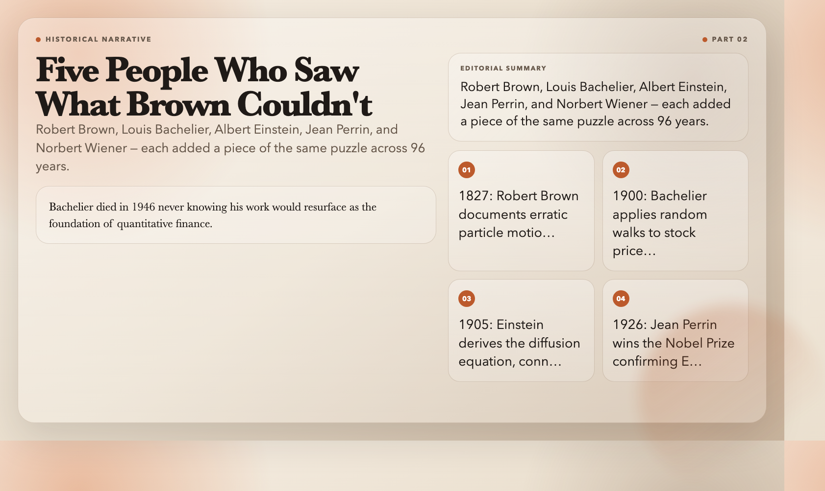
Robert Brown, 1827

Brown documented what he saw with meticulous precision: tiny particles suspended in water moved in “rapid but irregular” paths. He tested inorganic particles to rule out life as the cause. He failed to explain it. The phenomenon carried his name anyway.

Louis Bachelier, 1900

Bachelier was 23 when he submitted Théorie de la Spéculation to the University of Paris. He modeled stock price changes as a random walk. The French academy gave his work a passing grade but no standing. The Paris Bourse ignored it entirely. Bachelier died in 1946, never knowing his work would resurface as the foundation of quantitative finance. His 1900 PhD thesis was rediscovered in 1960.

Albert Einstein, 1905

The same year Einstein published special relativity, he published a paper explaining Brownian motion using kinetic theory. He derived a specific prediction: ⟨x²⟩ = 2Dt — the mean square displacement grows linearly with time, proportional to the diffusion coefficient. He showed that measuring D would yield Avogadro’s number. He was right. Jean Perrin measured it and won a Nobel Prize with it.

Jean Perrin, 1926

Perrin ran years of painstaking experiments on suspended particles. He counted, measured, averaged. His results matched Einstein’s predictions within 2%. “The reality of molecules is now beyond doubt,” he wrote. He won the Nobel Prize in Physics in 1926. His book Les Atomes converted the last serious skeptics of atomic theory.

Norbert Wiener, 1923

Wiener constructed a rigorous mathematical framework for Brownian motion. He defined the Wiener process with precise measure-theoretic foundations. His work became the backbone of Itô calculus and stochastic differential equations. He was also famously absent-minded and once reportedly showed up to a lecture he wasn’t scheduled to give.

The Visualization: Three Modes, One Equation

The Brownian Motion & Random Walk visualization runs in your browser. Three modes, one core equation, five preset experiments.

Physics Mode

Start 50 particles at the origin. Set D = 1.0, dt = 0.01. Press play.

Watch two things simultaneously: individual particles zigzag randomly, and the collective histogram morphs into a Gaussian bell curve. The curve sharpens over time. The spread grows as √t.

The Einstein Relation experiment: Run 50 particles for T = 10.0 (1000 steps). Open the Mean Square Displacement plot. The regression slope equals 2D. Set D = 1.0, expect slope ≈ 2.0. If your simulation gives 1.95–2.05, Einstein’s prediction is confirmed in your browser.

This is the diffusion equation — the same math that predicts how ink spreads in water, how heat distributes through metal, and how pollutants disperse in air.

Finance Mode

Toggle to Finance Mode. The same Gaussian process becomes a stock price model.

Set S₀ = 100, σ = 0.2, μ = 0.08 (annual). Simulate 50 price paths for T = 1 year. You see a fan of possible prices — some end at 140, some at 70. The distribution is log-normal (log prices are normal). This is Geometric Brownian Motion (GBM), the same model Black and Scholes used in 1973.

The bear market experiment: Set μ = -0.05, σ = 0.3. Run 100 paths. What fraction end below S₀ = 100? Count them. Now set μ = 0.15, σ = 0.2. Run again. The shift in probability of profit is visible in seconds.

The Black-Scholes experiment: Set S₀ = 100, K = 100, T = 1 year. Simulate 1000 paths. Compute the average call payoff: max(S_T – K, 0). Discount at r = 0.05. The result should be approximately 10.45 (the closed-form Black-Scholes value for these parameters). The simulation converges to the analytical solution as path count increases. This is Monte Carlo method in action.

Math Mode

The pure mathematics. Here you see the Central Limit Theorem operating directly.

Take the simplest random process imaginable: each step, move ±1 with equal probability. No physics, no finance. Just the math.

Run 200 particles for 500 steps each. The histogram of final positions is a bell curve. Run 1000 particles. Still a bell curve. Change the step distribution — introduce a slight bias (51% up, 49% down). Run again. After enough steps, you still get a Gaussian. The CLT doesn’t care what the underlying distribution is — it always produces the same output.

This is why Brownian motion is Gaussian. Not by assumption. By mathematical law.

The √t Law: What It Means in Practice

Here is a number worth remembering:

⟨x²⟩ = 2Dt means that to double the typical spread, you need four times the time.**

This is not intuitive. Most people guess 2x time → 2x spread. The math says 4x time → 2x spread. The spread grows as the square root of time.

In finance, this is why annualizing volatility is not a simple division. A stock with 20% daily volatility does not have 20% × 252 ≈ 5040% annual volatility. It has 20% × √252 ≈ 317% annual volatility. The square root correction is the difference between a reasonable estimate and financial nonsense.

The same law governs:
– How quickly heat spreads in a metal rod
– How far a molecule travels in a given time
– How uncertainty in a measurement grows with repeated sampling

Where the Model Breaks Down

Brownian motion is continuous but nowhere differentiable. Its paths are infinitely rough — no derivative exists at any point. Real particles have smooth trajectories. The resolution is scale: millions of molecular collisions per second average into apparent smoothness. The model is an approximation that works because the molecular timescale is far shorter than the observational timescale.

More importantly: real markets are not stationary. GBM assumes volatility is constant. Real volatility clusters, jumps, and follows regimes. Long-Term Capital Management collapsed in 1998 partly because their models assumed mean reversion in credit spreads. The spreads didn’t mean-revert. The fund lost $4.6 billion in six weeks.

Models like stochastic volatility (Heston, 1993), jump-diffusion (Merton, 1976), and fractional Brownian motion try to address these failures. None have displaced GBM as the industry workhorse. It’s the simplest model that’s “right enough” for most applications — which is both its strength and its danger.

Try It Now

The Brownian Motion & Random Walk visualization is live in your browser. No install. No account. Three modes, five preset experiments, and real mathematical machinery running in real time.

Start with Physics Mode. Run the Einstein experiment. Watch the Gaussian emerge. Then switch to Finance Mode and price an option with your own Monte Carlo simulation.

When the bell curve appears from pure randomness — 50 particles all making independent, aimless ±1 steps — you’ll understand why five brilliant minds couldn’t let this idea go.

The randomness you’re watching is the same math that prices your options.

Tags: Brownian Motion, Random Walk, Stochastic Processes, Geometric Brownian Motion, Black-Scholes, Monte Carlo Simulation, Physics Visualization, Finance, Mathematical Finance, Diffusion
Featured Image: Brownian Motion & Random Walk — Interactive Visualization