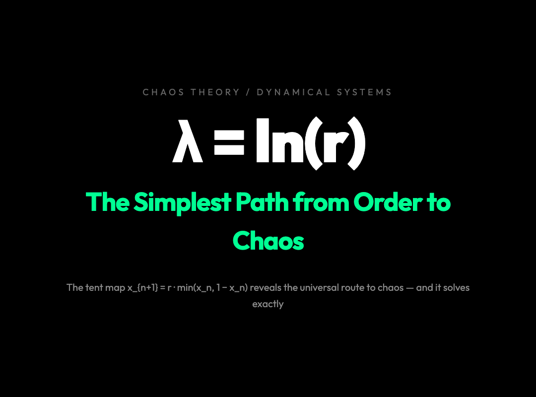
The Simplest Equation That Proves Chaos Has a Hidden Order

The tent map looks innocent. It lives inside a single line of math:

x_{n+1} = r · min(x_n, 1 − x_n)

If you’ve encountered the logistic map in any chaos theory course, this formula should feel strangely familiar — because it is, in every way that matters, the logistic map’s twin. Just with its nonlinear “crease” smoothed into a sharp V-shape.

And that sharp V is precisely what makes the tent map so clarifying. When the math has no curves to hide behind, the path from order to chaos becomes impossible to miss.

What the Equation Actually Does

The tent map takes a number between 0 and 1, then maps it to a new number using a single parameter r (between 0 and 2).

Visually, it folds the unit interval in half like a tent — the left side rises linearly from 0 to a peak at r/2, then the right side falls back to 0.

At r = 1, the whole system collapses to a single point: every starting value converges to 0.

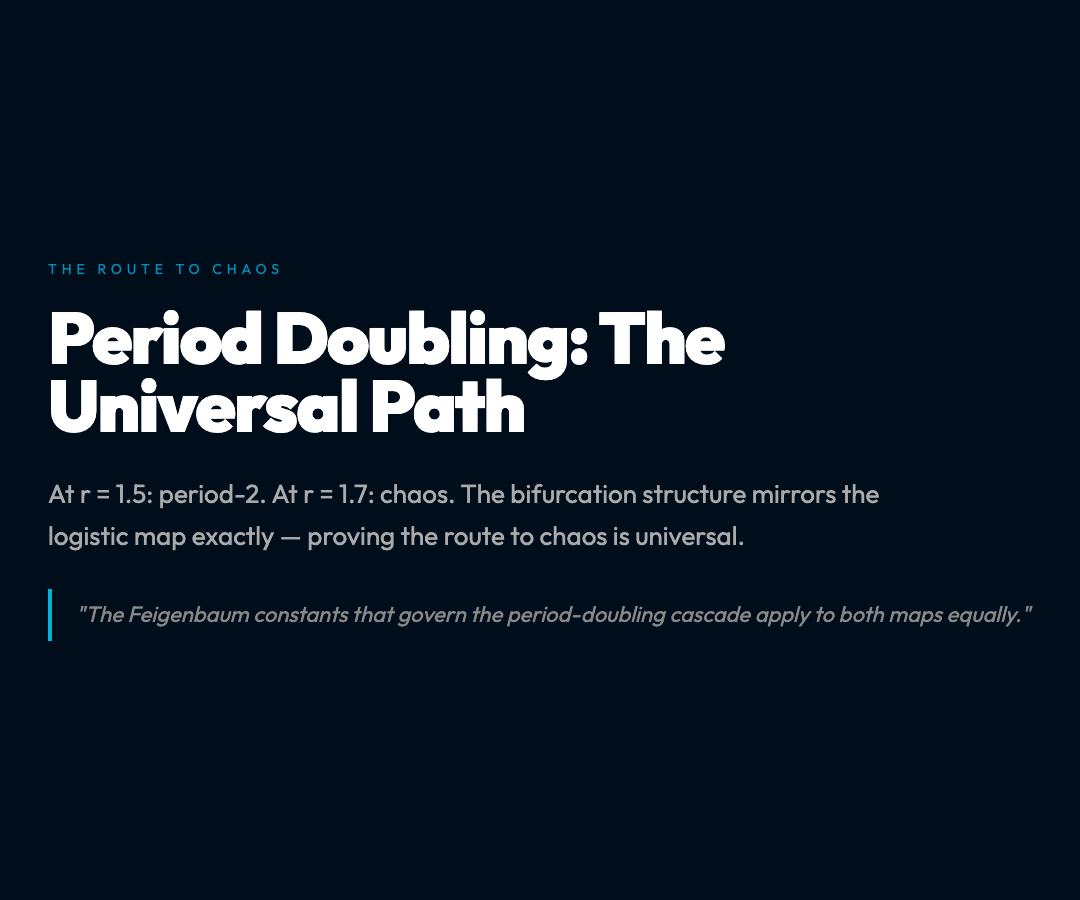
At r = 1.5, you get period-2 oscillations — the system bounces between two values.

At r = 1.7, the bounces become irregular. Not random, but not predictable either.

At r = 2, you get full chaos: the system generates a sequence that never repeats, never settles, and depends so sensitively on the starting value that two trajectories starting just 0.0001 apart will, after 30 iterations, be on opposite ends of the interval.

This is the hallmark of chaos — sensitive dependence on initial conditions — and it emerges from one of the simplest nonlinear systems imaginable.

The Bifurcation Diagram: Order and Chaos in One Image

The most revealing way to see the tent map’s behavior is through its bifurcation diagram, which plots every steady-state value the system reaches as the parameter r sweeps from 0 to 2.

At low r, the diagram shows a single line — the system converges to one value.

Around r = 1, the line splits into two: period doubling has begun.

As r increases past 1.3, the two lines split into four. Then eight. Then sixteen.

By r ≈ 1.7, the lines have become a haze — a signature fingerprint of chaos.

Here’s what makes this remarkable: the bifurcation structure of the tent map is mathematically identical to the bifurcation structure of the logistic map, the most famous equation in chaos theory. Different equations, different functional forms, but the same universal route from order to chaos through period-doubling.

This is one of the great discoveries of dynamical systems theory: the path to chaos is universal. The Feigenbaum constants — the precise ratios governing the period-doubling cascade — apply to both maps equally.

Lyapunov Exponent: Measuring Chaos Precisely

One of the tent map’s superpowers is that its Lyapunov exponent — the primary measure of chaotic behavior — has an exact analytical formula:

λ = ln(r)

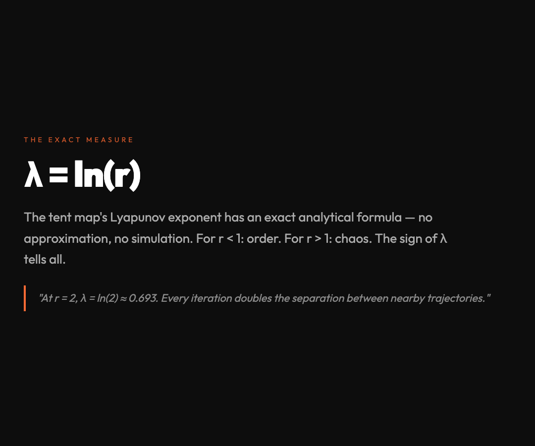
For r < 1: λ < 0, and the system converges (negative exponent = order).

For r = 1: λ = 0, the critical boundary between order and complexity.

For r > 1: λ > 0, and the system is chaotic. The larger r, the more rapidly trajectories diverge.

At r = 2, λ = ln(2) ≈ 0.693. Every iteration doubles the separation between nearby trajectories, on average. After 10 iterations, trajectories that started 0.0001 apart are separated by about 10 centimeters on the unit interval. After 30, they’re effectively uncorrelated.

The tent map lets you see this directly in its multi-orbit view, which plots several trajectories with microscopically different starting values side by side. For r values above 1, watch how the trajectories start aligned and then fan apart into apparent disorder.

Why the Tent Map Matters More Than It Looks

The tent map is often taught as a “simpler version” of the logistic map. But that framing undersells it.

Because the tent map is piecewise linear, every calculation involving it is tractable. The Lyapunov exponent isn’t an approximation — it’s exact. The bifurcation diagram isn’t a numerical simulation — it’s a direct consequence of the map’s geometry.

This makes the tent map a proof engine for chaos theory. When you want to establish a result about chaotic systems — properties of Lyapunov exponents, the structure of strange attractors, the statistics of return times — you often prove it first for the tent map because you can solve it by hand.

The tent map is to chaos theory what the harmonic oscillator is to classical mechanics: the irreducible simplest case that reveals the essential physics, stripped of all complications that don’t bear on the core phenomenon.

Explore It Live

The Tent Map Visualization at ElysiaTools lets you manipulate the parameter r in real time and watch the bifurcation diagram update live. Switch between the time series view, the cobweb diagram (which shows the folding geometry directly), the bifurcation diagram, and the multi-orbit view.

Pay attention to what happens as you sweep r past 1.7. The system doesn’t suddenly become “random.” It was always deterministic — it always follows the exact same rule. But the rule produces behavior that is, for all practical purposes, indistinguishable from randomness.

That’s what chaos really means: not a failure of determinism, but the existence of deterministic systems whose long-term behavior cannot be predicted in practice — no matter how precisely you know the starting conditions.

The tent map makes this philosophical shock as concrete and visual as it can possibly be.