The Heisenberg Uncertainty Principle of Sound: Why You Can’t Have Perfect Time and Frequency Resolution
In 1927, Werner Heisenberg discovered something unsettling about the quantum world: you cannot simultaneously know a particle’s exact position and momentum. The more precisely you measure one, the less you know about the other.
What Heisenberg didn’t know is that the same principle governs every audio file on your hard drive.
The Problem With Waveforms
When you open an audio file in any standard editor, you see a waveform — a two-dimensional representation of pressure variation over time. It tells you when something happened, but it tells you almost nothing about what happened.
Look at a waveform of a bird call. You can see it occurred at second 2.3. But you cannot tell whether it was a high-pitched chirp or a low hoot. Look at a waveform of someone saying “ba” versus “da.” Visually, they may look nearly identical — yet your brain instantly hears the difference.
The reason: waveforms collapse all frequency information into a single dimension. The ear doesn’t work that way. The ear decomposes sound into frequencies — it hears pitch, timbre, resonance. The waveform shows you time. The brain wants frequency.
The Spectrogram: Slicing Sound Into Time-Frequency Cells
A spectrogram solves this. Instead of plotting amplitude over time, it plots energy over both time and frequency simultaneously — a three-dimensional landscape where x-axis is time, y-axis is frequency, and color intensity represents how much energy lives at each time-frequency point.
The result is a heatmap. Silence appears dark. A pure 440 Hz tone appears as a bright horizontal line. A chirp — a sound that sweeps from low to high frequency — appears as a bright diagonal stripe.
Suddenly, sound becomes visible.
But here’s where it gets interesting.
The Fundamental Trade-off: Window Size
To build a spectrogram, you can’t just look at an entire audio file all at once. You have to cut it into small windows, compute a Fourier transform on each window, then stitch the results together. And this is where Heisenberg’s ghost reappears.
The window size — how much audio you analyze at once — controls a fundamental trade-off:
Large window: You get excellent frequency resolution. You can precisely distinguish two nearby frequencies, say 440 Hz and 442 Hz. But because you’re averaging over a long time segment, you lose time resolution — you can’t pinpoint when a frequency appeared with precision.
Small window: You get excellent time resolution. You can precisely locate the moment a note began. But because you’re averaging over so little time, the frequency estimate becomes fuzzy — you lose the ability to distinguish nearby frequencies.
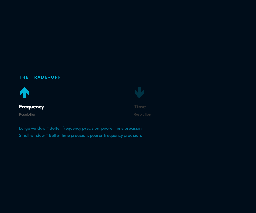
This is not a limitation of our instruments. It is a mathematical certainty, as fundamental as the speed of light. The product of time resolution and frequency resolution has a minimum value. You cannot beat it. You can only choose your compromise.
In physics, this is called the uncertainty principle. In signal processing, it has a different name but the same essence: the Short-Time Fourier Transform (STFT) obeys the same trade-off.
Why This Matters in the Real World
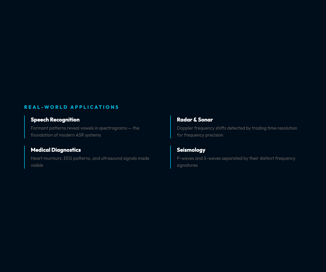
Speech recognition. When linguists first looked at spectrograms in the 1950s, they discovered something remarkable: vowel sounds produce bright horizontal bands called formants — specific frequency resonances that characterize each vowel. “EE” has formants around 300 Hz and 2500 Hz. “OO” has formants around 300 Hz and 900 Hz. A spectrogram doesn’t just show you sound. It reveals the phonetic structure of speech. This is how modern speech recognition systems were born.
Music production. Producers use spectrograms to identify frequency clashes between instruments. When the kick drum and bass guitar occupy the same frequency range, they muddle each other. A spectrogram makes this conflict visible as overlapping horizontal stripes — a spatial problem with a spatial solution: carve out different frequency bands for each instrument.
Radar and sonar. When a radar pulse bounces off a moving aircraft, its frequency shifts — the Doppler effect. But a stationary object and a slowly moving object produce very similar shifts. The solution: longer observation windows for finer frequency resolution, at the cost of slower update rates. This trade-off appears in every radar system ever built.
Medical diagnostics. Heart murmurs produce distinctive frequency signatures. EEG patterns — the electrical activity of your brain — show different frequency bands (alpha, beta, theta, delta) associated with different mental states. Spectrograms convert these invisible electrical patterns into visible maps, letting clinicians see what the ear cannot parse.
Seismology. Earthquakes produce P-waves and S-waves that travel at different speeds and frequencies. Spectrograms of seismograph readings help geologists distinguish these overlapping signals, estimate the earthquake’s depth, and assess its magnitude.
The Tool: Spectrogram Analyzer
The Spectrogram Analyzer on ElysiaTools lets you interact with this trade-off directly.
You can generate test signals — a pure sine wave, a square wave, a frequency chirp, or white noise — and watch how each appears in the spectrogram. You can upload your own audio file. You can adjust the window size and immediately see the resolution trade-off: larger windows stretch the bright features horizontally (better frequency precision), smaller windows compress them vertically (better time precision).
The educational panel explains the STFT formula, the role of window functions in reducing spectral leakage, and the applications across speech, music, radar, and medicine.
The core interaction is simple: move the window size slider and watch the spectrogram blur and sharpen along one axis or the other. In thirty seconds of experimentation, you develop an intuition for a trade-off that took physicists decades to formalize.
What You Can’t Beat
Heisenberg’s original principle was controversial because it suggested that nature itself has limits — that no amount of cleverness can overcome certain constraints. The time-frequency trade-off in spectrograms carries the same implication.
No algorithm, no machine, no future technology can produce a spectrogram with simultaneously perfect time and frequency resolution. This is not a hardware limitation. It is a property of waves themselves. The Fourier transform is doing the mathematics of wave decomposition, and waves resist being localized in both time and frequency simultaneously.
What you can do is choose your compromise deliberately. A music producer might choose a large window to see precise frequency details. A radar engineer might choose a small window to track fast-moving targets. A doctor might choose an intermediate window to balance clarity and responsiveness.
The spectrogram doesn’t give you the answer. It gives you the trade-off — and lets you decide what matters most.
The next time you see a sound visualized, whether it’s a spectrogram in a music app, a frequency analyzer in a podcast editor, or an emergency alert on your phone, remember: you’re looking at a universe that obeys Heisenberg’s rules, even when there’s no quantum mechanics in sight. Sound is a wave. Waves don’t give you everything at once.
And that’s precisely what makes them interesting to look at.