The Beautiful Math Behind the Shapes That Appear When Two Waves Collide
In 1857, the American mathematician Nathaniel Bowditch watched a point being pulled simultaneously by two perpendicular forces — one oscillating slowly, one fast — and traced what emerged on paper. The shape that appeared was neither a circle nor an ellipse. It was something stranger: a looping, intricate curve that shifted as the relative frequencies and phases changed. Jules Antoine Lissajous would publish the full mathematical analysis a year later, giving his name to a phenomenon that physicists, engineers, and mathematicians still find endlessly surprising.
The equations are simple to write down:
x(t) = A₁ · sin(ω₁t + δ) y(t) = A₂ · sin(ω₂t)
Two sine waves at right angles. Two frequencies. One phase difference. The result is a Lissajous figure — and the variety of shapes hidden in that simple system is far richer than you would expect.
The Oscilloscope Connection
If you ever worked with an oscilloscope in X-Y mode, you have generated Lissajous figures. The horizontal and vertical deflection plates of a CRT display are driven by separate signals. Feed two sine waves of different frequencies into each axis and the screen traces a Lissajous figure in real time.
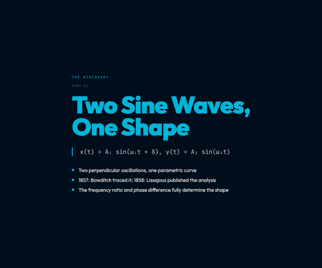
This was not merely a curiosity. Engineers used these patterns to measure the frequency ratio between two signals with remarkable precision. If you knew one frequency and counted the number of lobes — the closed “loops” in the pattern — you could read off the frequency ratio directly from the screen. A figure with 3 horizontal lobes and 2 vertical lobes meant a 3:2 frequency ratio. Clean, simple, and visible without any digital instrumentation.
The stability of the pattern was itself diagnostic. A perfectly stable figure meant the two frequencies were locked in an exact integer ratio. A wandering, non-repeating trace meant the ratio was irrational — the two frequencies were incommensurate, and the pattern would never close.
The Frequency Ratio: Why 1:1, 1:2, 2:3 Look So Different
The key to understanding Lissajous figures is the frequency ratio ω₁:ω₂.
When the ratio is 1:1, you get the simplest family. At δ = 0° or 180°, you get a straight line at 45°. At δ = 90°, you get a circle. At any other phase difference, you get an ellipse. This is not new — it’s just the familiar result of adding two sinusoidal motions at right angles. The entire 1:1 family is well-described by the single parameter δ.
When the ratio jumps to 1:2, the first genuinely new behavior appears. A 1:2 Lissajous figure with δ = 90° produces the classic figure-8 — the y-axis completes two oscillations in the same time the x-axis completes one. The two loops are equal in size because the phase relationship is symmetric. Change the phase difference and the loops distort, asymmetrically at first, then merge into a single parabola-like curve before reforming as the mirror image of the original figure-8.
At 2:3, the pattern acquires three lobes horizontally and two vertically. It is visually more complex but still fully determined by the phase difference. Sweep through δ from 0° to 360° and the pattern morphs continuously through a recognizable sequence of shapes.
At 3:4 and beyond, the patterns grow proportionally more intricate. A 3:4 figure has three lobes in one direction and four in the other. A 5:4 figure looks almost like a tangled braid. The complexity grows because the pattern only closes after a full cycle of the frequency ratio — for ω₁:ω₂ = 5:4, you need 5 x-axis cycles and 4 y-axis cycles before the point returns to its starting position.
The Role of Phase: Why δ Matters as Much as the Frequency
Most introductions to Lissajous figures emphasize the frequency ratio, but the phase difference δ is equally constitutive. At ω₁:ω₂ = 1:1, varying δ from 0° to 360° traces a complete morphological sequence: a line at 0°, then an ellipse that opens into a circle at 90°, then back through a narrower ellipse to a line at 180° (now oriented the opposite way), then an ellipse rotating in the opposite sense, back to a circle at 270°, and finally to the original line at 360°.
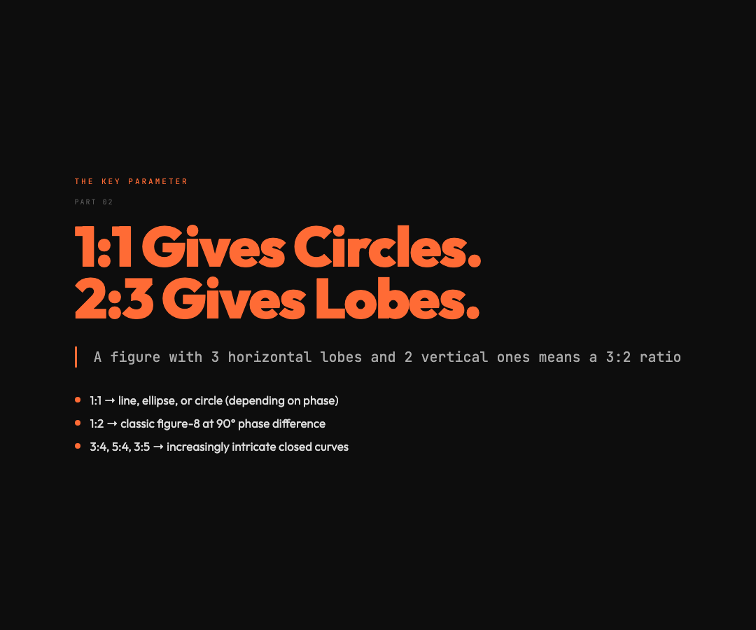
This is a complete classification of all possible outcomes from a single frequency ratio — and it is determined entirely by the phase. The same sensitivity applies at every frequency ratio. A 1:2 figure at δ = 0° looks nothing like a 1:2 figure at δ = 90°. The phase is not a minor correction. It is a free parameter that fully specifies the shape.
The Interactive Visualization: Seeing the Full Parameter Space
The Lissajous Figures visualization on ElysiaTools lets you explore this parameter space directly. You control:
– ω₁ and ω₂: the two frequencies (expressed as a ratio) – A₁ and A₂: the amplitudes on each axis – δ: the phase difference – Animation speed: watch the point trace the figure in real time
The preset buttons take you immediately to the classic cases — the circle at 1:1 with 90° phase, the figure-8 at 1:2, the complex 2:3 and 3:4 patterns. But the real insight comes from turning the knobs yourself. Watching the figure-8 distort continuously as you sweep δ from 0° to 90° gives you a concrete sense of what the phase parameter actually does — something no static diagram can convey.
The trail length control is particularly revealing. Set it short and you see the point’s trajectory as it builds the figure — you can watch the path cross itself in a specific order, which gives intuition for why certain frequency ratios produce loops and others produce more tangled webs.
The Physics Behind the Pattern
Lissajous figures appear wherever two orthogonal oscillatory processes interact. They are not merely a laboratory curiosity:
– Acoustics: When two tuning forks vibrate at slightly different frequencies and are held at right angles to each other, the combined motion of their sound waves produces Lissajous patterns in the air. – Electronics: The X-Y mode on oscilloscopes was historically the primary tool for comparing frequencies and measuring phase differences between signals. – Mechanics: The motion of a mass on two perpendicular springs, or a pendulum with two perpendicular swing planes, traces Lissajous figures. – Optics: The interference pattern formed by two coherent beams arriving at slightly different angles produces intensity distributions with Lissajous-like structure.
The common thread is superposition — two oscillations, one physical system, perpendicular in some relevant degree of freedom. The mathematics of superposition produces the patterns without requiring any special interaction between the two waves.
The Closed Pattern Condition: When Does the Figure Repeat?
Not every pair of frequencies produces a closed Lissajous figure. The figure closes — returning to its starting point and repeating — if and only if the frequency ratio ω₁:ω₂ is a rational number (a ratio of integers).
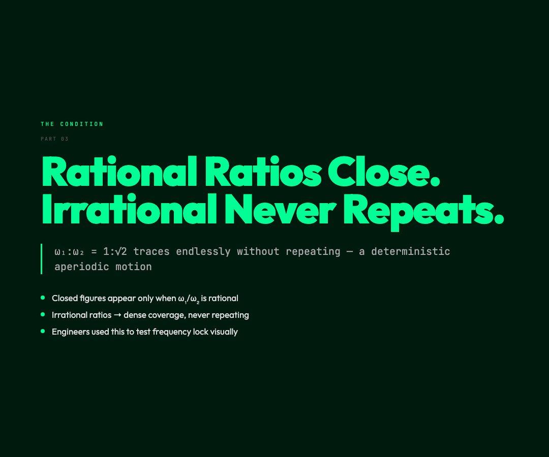
If ω₁:ω₂ = 1:√2 (an irrational ratio), the pattern never closes. The point traces endlessly without repeating, covering the rectangular region densely. This is a genuinely aperiodic motion that arises from a perfectly deterministic system — no randomness, no noise, just two pure sine waves with incommensurate frequencies.
This sensitivity to rational versus irrational frequency ratios was historically important: it gave physicists and engineers a visual test for whether two frequencies were locked in a rational relationship. If the oscilloscope trace was stable and closed, the ratio was rational. If it wandered, it was not.
What the Lissajous Figure Teaches
The remarkable thing about Lissajous figures is not that they are complicated. It is that they are fully deterministic yet visually surprising. Two simple equations, one phase parameter, and the variety spans lines, circles, ellipses, figure-8s, and increasingly elaborate closed curves with no upper bound on their complexity.
The parameter space is small — three continuous parameters (ω₁:ω₂, δ, and the amplitude ratio) — but it generates an infinite set of qualitatively distinct shapes. This is the signature of a rich mathematical structure, and it is why Lissajous figures remain a useful pedagogical tool for teaching parametric curves, phase relationships, and the behavior of oscillatory systems.
They are also simply beautiful. The figure-8 is clean and symmetric. The 3:4 figure looks like a precision-machined mechanical part. The 5:4 figure resembles a folded ribbon. These are not decorative shapes imposed on the mathematics — they emerge directly from the sinusoidal parametric equations.
Open the visualization, set ω₁:ω₂ to 3:5, sweep δ from 0 to 360°, and watch what happens. The shape that appears is not one you would easily predict from the equations alone. That gap between prediction and observation — between the simple algebra and the complex geometry — is where the interesting physics lives.
Try the Lissajous Figures visualization and explore the full parameter space for yourself.